PCA of Standardized Rasch Residuals

Fits a Rasch model (eRm::RM() for dichotomous data, eRm::PCM() for polytomous data — chosen automatically), extracts standardized residuals via eRm::itemfit()$st.res, and runs an unrotated principal-component analysis on those residuals via stats::prcomp(). The function reports the top n_components eigenvalues and their proportions of unexplained variance, and optionally compares the first-contrast eigenvalue against a simulation-based bound from RMdimResidualPCACutoff.

Usage

RMdimResidualPCA(data, cutoff = NULL, n_components = 5L, output = "kable")

Arguments

data: A data.frame or matrix of item responses. Items must be scored starting at 0 (non-negative integers). Rows with any NA are dropped before PCA, since prcomp() does not accept missing values.
cutoff: Optional. The list returned by RMdimResidualPCACutoff (its suggested_cutoff is used), or a single numeric value to use as the cutoff directly. When provided, the result includes a Flagged column (logical: is the eigenvalue above the simulated bound?) and the kable caption notes the cutoff.
n_components: Integer. Number of eigenvalues to report. Capped at the number of items. Default 5.
output: Character. "kable" (default) for a formatted knitr::kable() table, "dataframe" for the underlying data.frame, or "loadings" for a ggplot of PC1 loadings against item locations (similar in spirit to the loadings-by-location plot used in easyRasch::RIloadLoc).

Value

If output = "kable": a knitr_kable object with columns Component, Eigenvalue, Proportion of variance (and Flagged when cutoff is provided). The caption gives the variance partition (% of total observed variance explained by measures vs. unexplained), the model fitted, sample size, and cutoff metadata if applicable.
If output = "dataframe": a data.frame with columns Component, Eigenvalue, Proportion_of_variance (and Flagged when cutoff is provided). The variance partition is attached as the "variance_partition" attribute — a list with elements total, explained, unexplained, pct_explained, pct_unexplained, n_persons. Access via attr(result, "variance_partition").
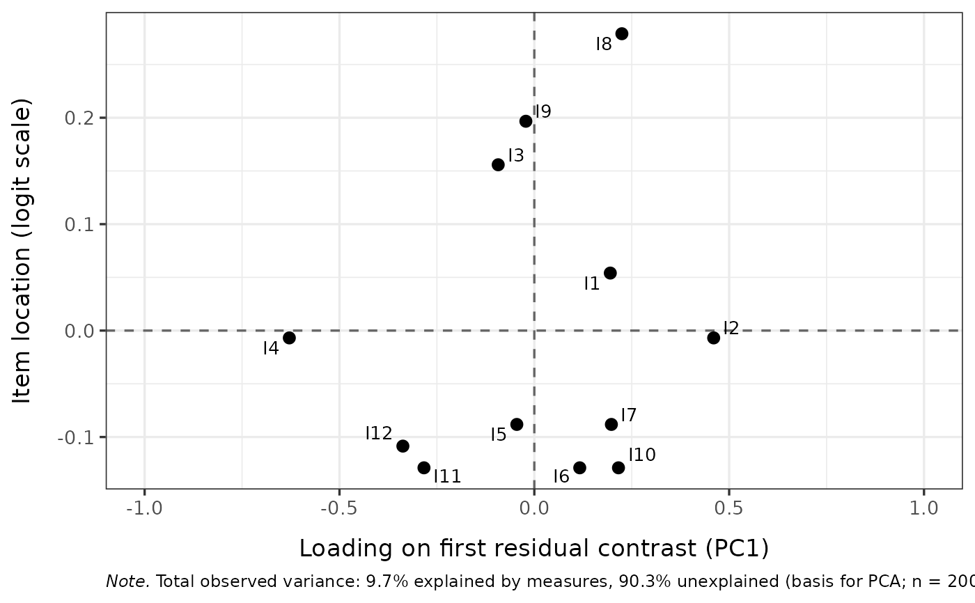
If output = "loadings": a ggplot showing each item's PC1 loading on the x-axis and Rasch item location on the y-axis, with dashed reference lines at zero, and the variance partition in the figure caption. Item names are labelled via ggrepel::geom_text_repel() when ggrepel is installed; otherwise plain geom_text().

Details

Rule-of-thumb thresholds for the first-contrast eigenvalue (e.g., the "> 2" heuristic occasionally cited from Winsteps documentation) are not reliable indicators of multidimensionality; the first-contrast eigenvalue under a correctly fitting unidimensional model varies systematically with sample size, test length, and item-parameter spread. Empirical (simulated) bounds tailored to the data structure should be used instead — see RMdimResidualPCACutoff, and Chou & Wang (2010) for the underlying simulation argument.

The PCA is performed on the standardized residuals returned by eRm::itemfit()$st.res, which are (observed - expected) / sqrt(var) under the Rasch model. The reported eigenvalues are unrotated; rotation is appropriate for interpreting a multidimensional solution but obscures the dominant first contrast that dimensionality assessment is concerned with.

Item locations on the loadings plot are computed as the per-item mean of Andrich thresholds for polytomous data (PCM) or as -beta for dichotomous data (RM).

The variance partition follows Linacre's CML/MLE convention: per-item observed variance is compared to per-item expected variance under the fitted model, summed across items. Expected scores are computed from MLE person locations (via eRm::person.parameter()) and the CML item parameters from eRm::RM() / eRm::PCM(). Persons with extreme raw scores (no finite MLE theta) are excluded from the partition, matching the sample used by eRm::SepRel() and the PCA itself.

References

Chou, Y.-T., & Wang, W.-C. (2010). Checking dimensionality in item response models with principal component analysis on standardized residuals. Educational and Psychological Measurement, 70(5), 717-731. doi:10.1177/0013164410379322

Examples

# \donttest{
set.seed(1)
dat <- as.data.frame(
  matrix(sample(0:1, 200 * 12, replace = TRUE), nrow = 200, ncol = 12)
)
colnames(dat) <- paste0("I", 1:12)

# Default kable output
RMdimResidualPCA(dat)
#> 
#> 
#> Table: Rasch model (200 complete cases, 12 items). Total observed variance: 9.7% explained by measures, 90.3% unexplained
#> (basis for PCA; n = 200 non-extreme cases).
#> 
#> |Component | Eigenvalue| Proportion of variance|
#> |:---------|----------:|----------------------:|
#> |PC1       |      1.464|                  0.121|
#> |PC2       |      1.425|                  0.118|
#> |PC3       |      1.281|                  0.106|
#> |PC4       |      1.155|                  0.096|
#> |PC5       |      1.125|                  0.093|

# PC1 loadings vs item location plot
RMdimResidualPCA(dat, output = "loadings")


# Simulation-based cutoff (use 250+ iterations in real analyses)
bound <- RMdimResidualPCACutoff(dat, iterations = 50, parallel = FALSE, seed = 1)
RMdimResidualPCA(dat, cutoff = bound)
#> 
#> 
#> Table: Rasch model (200 complete cases, 12 items). Total observed variance: 9.7% explained by measures, 90.3% unexplained
#> (basis for PCA; n = 200 non-extreme cases). First-contrast cutoff = 1.657 based on 50 simulation iterations (99th percentile).
#> 
#> |Component | Eigenvalue| Proportion of variance|Flagged |
#> |:---------|----------:|----------------------:|:-------|
#> |PC1       |      1.464|                  0.121|FALSE   |
#> |PC2       |      1.425|                  0.118|FALSE   |
#> |PC3       |      1.281|                  0.106|FALSE   |
#> |PC4       |      1.155|                  0.096|FALSE   |
#> |PC5       |      1.125|                  0.093|FALSE   |
# }