A Rasch analysis workflow with easyRasch2 • easyRasch2

Overview

This vignette walks through the steps of a Rasch analysis using data from the nine-item Patient Health Questionnaire (PHQ-9; Kroenke et al. (2001)). The example follows the four psychometric criteria proposed by Christensen et al. (2021) for the validation of patient-reported outcome measures (PROMs):

Unidimensionality — the items measure a single latent construct.
Local independence — after conditioning on the latent trait, item responses are independent of each other.
Ordered response category thresholds (monotonicity) — moving up the latent trait increases the probability of higher categories.
Invariance / no DIF — item parameters are the same across relevant external groups (e.g. gender).

We then move on to complementary descriptors that are commonly reported alongside the four criteria above:

Targeting — how well person and item locations overlap on the latent continuum.
Reliability — how precisely the scale separates respondents.
Person fit — unexpected response patterns.
Item and person parameters — estimates for reuse in scoring.

For a more extensive treatment of Rasch analysis in R, see https://pgmj.github.io/raschrvignette/RaschRvign.html. For a Bayesian sibling package, see https://pgmj.github.io/easyRaschBayes/.

NOTE: all simulation-based functions use a low number of iterations to make this vignette render faster. You should use more iterations for actual analysis work. For most methods, 500-1500 will be useful, except for conditional infit, where lower numbers can be optimal, depending on sample size (Johansson 2025). If you plan to use p_value = TRUE, use at least 1000 iterations.

To get faster simulations, please make use of options(mc.cores = 4), where 4 should be replaced with the number of high performance CPU cores your computer has available. This setting is automatically applied by all functions that can use parallel processing.

Data

The bundled phq9 dataset is a 600-respondent random subsample of the PHQ-9 module from the U.S. National Health and Nutrition Examination Survey (NHANES, September 2024 release) with complete responses on all nine items. NHANES microdata are released to the public domain by the U.S. federal government.

library(easyRasch2)
data(phq9)
items <- phq9[, 1:9]   # 9 item columns, scored 0..3

# add item information
item_desc <- c(
  "Little interest or pleasure in doing things",
  "Feeling down, depressed, or hopeless",
  "Trouble falling or staying asleep, or sleeping too much",
  "Feeling tired or having little energy",
  "Poor appetite or overeating",
  "Feeling bad about yourself - or that you are a failure or have let yourself or your family down",
  "Trouble concentrating on things, such as reading the newspaper or watching television",
  "Moving or speaking so slowly that other people could have noticed",
  "Thoughts that you would be better off dead or of hurting yourself in some way"
)

item_resp <- c("Not at all","Several days","More than \nhalf the days","Nearly every day")

str(items)
#> 'data.frame':    600 obs. of  9 variables:
#>  $ q1: int  3 0 1 2 3 3 1 3 2 1 ...
#>  $ q2: int  3 0 2 3 3 3 1 3 2 0 ...
#>  $ q3: int  3 1 3 0 3 1 0 3 2 0 ...
#>  $ q4: int  3 1 3 2 3 3 1 3 2 0 ...
#>  $ q5: int  3 0 3 2 3 2 0 1 2 0 ...
#>  $ q6: int  3 2 3 2 3 2 2 3 3 0 ...
#>  $ q7: int  3 3 3 2 3 2 2 3 3 0 ...
#>  $ q8: int  1 0 2 0 3 3 0 0 1 0 ...
#>  $ q9: int  3 0 0 2 3 1 2 0 0 0 ...
summary(rowSums(items))
#>    Min. 1st Qu.  Median    Mean 3rd Qu.    Max. 
#>    0.00   10.00   16.00   15.41   21.00   27.00
table(phq9$gender, useNA = "ifany")
#> 
#> Female   Male   <NA> 
#>    426    143     31
summary(phq9$age)
#>    Min. 1st Qu.  Median    Mean 3rd Qu.    Max. 
#>   15.00   26.00   33.00   36.06   44.00   85.00

Descriptive plots

Before fitting any model it is worth eyeballing the response distributions:

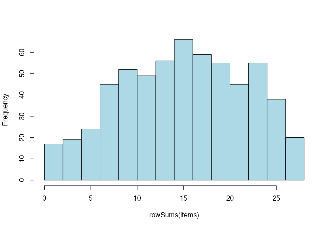
hist(rowSums(items), col = "lightblue", main = "", xlab = "Ordinal sum scores")

Figure 1. Histogram of ordinal sum scores

RMplotBar(items, ncol = 2)

Figure 2. Faceted bar chart of response distributions

RMplotStackedbar(items, show_percent = TRUE)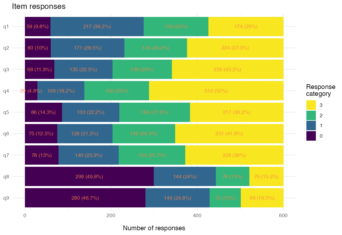

Figure 3. Stacked-bar response distribution

1. Unidimensionality

easyRasch2 provides several complementary unidimensionality diagnostics that can be combined for a robust conclusion:

item-level conditional infit MSQ statistics (Müller 2020)
item-level item-restscore associations with Goodman-Kruskal’s \gamma (gamma) (Kreiner 2011)
confirmatory factor analysis (CFA) with WLSMV estimator for ordinal data
principal components analysis (PCA) of the standardized residuals (Chou and Wang 2010)
Martin-Löf test with Monte-Carlo p-values (Christensen and Kreiner 2007)

Conditional infit MSQ

It is important to note that the RMitemInfit() function uses conditional infit, which is both robust to different sample sizes and makes ZSTD unnecessary (Müller 2020). Müller also questions the usefulness of outfit, and my simulation study (Johansson 2025) reached the same conclusion. Thus, outfit is not reported.

Conditional item infit mean-square statistics flag items whose response patterns deviate from the Rasch expectation. With RMitemInfitCutoff(), per-item highest-density intervals serve as the reference instead of rule-of-thumb cutoffs (Johansson 2025). Bootstrap p-values are also available via p_value = TRUE, with family-wise error rate (FWER; the default) or false discovery rate (FDR) correction.

NOTE: All functions that use simulation-based cutoffs (except RMitemInfitMI()) have an optional p_value = TRUE for their table outputs.

infit_cut <- RMitemInfitCutoff(items, iterations = 100, parallel = FALSE,
                           seed = 3)
RMitemInfit(items, cutoff = infit_cut)

MSQ values based on conditional estimation. n = 600 respondents. Cutoff values based on 100 simulation iterations (99.9% HDCI). Flagged: overfit = infit below range (more predictable); underfit = above range (noisier).
Item	Infit MSQ	Infit low	Infit high	Flagged	Relative location
q1	0.946	0.883	1.143		-0.56
q2	0.778	0.883	1.107	overfit	-0.76
q3	1.234	0.878	1.194	underfit	-0.83
q4	0.835	0.867	1.178	overfit	-1.48
q5	1.069	0.900	1.110		-0.58
q6	0.895	0.858	1.219		-0.76
q7	0.986	0.899	1.153		-0.66
q8	1.260	0.856	1.136	underfit	0.97
q9	1.315	0.842	1.199	underfit	0.79

You can also get a plot summarizing simulated and observed item infit, using RMitemInfitPlot(). Since conditional infit needs complete data, sibling functions that combine multiple imputation with conditional infit are useful when you have partial missingness: RMitemInfitMI() and RMitemInfitCutoffMI().

Based on the table, items 3, 8, and 9 underfit the Rasch model, while items 2 and 4 are overfit. Item 2 is “Feeling down, depressed, or hopeless”, which is a very general item in terms of measuring depression, so this is expected.

A low item fit value, often referred to as an item being “overfit” to the Rasch model, indicates that responses may be too predictable. This is often the case for items that are very general/broad in scope in relation to the latent variable. You will often find overfitting items to also have local dependence (residual correlations) issues with other items. Overfit may be likened to having a much stronger factor loading than other items in a confirmatory factor analysis or a higher level of discrimination in an Item Response Theory model with two or more parameters.

A high item fit value, often referred to as being “underfit” to the Rasch model, can indicate several things. Often underfit is due to multidimensionality or a question that is difficult to interpret and thus has noisy response data. The latter could for instance be caused by a question that asks about two things at the same time, or is ambiguous for other reasons.

Item-restscore

Item-restscore uses Goodman-Kruskal’s \gamma (gamma) and shows the expected and observed correlation between an item and a score based on the rest of the items (Kreiner 2011). Similarly, but inverted, to item infit, a lower observed correlation value than expected indicates underfit, that the item may not belong to the dimension. A higher than expected observed value indicates an overfitting and possibly redundant item. Overfitting items will often also show issues with local dependency.

Compared to infit, item-restscore more often flags overfit items (based on experience), and less often flags underfit items (based on a simulation study (Johansson 2025)).

RMitemRestscore(items)

Item-restscore associations. n = 600 respondents. Flagged (adj. p < .05): overfit = observed above expected (over-discrimination, often local dependence); underfit = below (under-discrimination, often multidimensionality/noise).
Item	Observed	Expected	Difference	Adj. p-value (BH)	Flagged	Rel. location
q1	0.66	0.62	0.041	0.210		-0.56
q2	0.72	0.62	0.103	0.000	overfit	-0.76
q3	0.57	0.63	-0.059	0.085		-0.83
q4	0.71	0.62	0.097	0.000	overfit	-1.48
q5	0.62	0.62	-0.001	0.968		-0.58
q6	0.69	0.63	0.065	0.021	overfit	-0.76
q7	0.64	0.62	0.020	0.476		-0.66
q8	0.55	0.63	-0.083	0.021	underfit	0.97
q9	0.59	0.64	-0.046	0.151		0.79

Similarly to infit, item-restscore found items 2 and 4 to be overfit and 8 to be underfit. It also found item 6 to be overfit. These methods are best used together.

CFA-based cutoffs for CFI / RMSEA and item loadings

RMdimCFACutoff() simulates data from a unidimensional PCM and fits a unidimensional ordinal CFA to each simulated dataset, building a parametric-bootstrap reference distribution for the model fit indices (SRMR, CFI, RMSEA) and for the per-item standardized factor loadings. It returns this simulation object; RMdimCFA() then fits the CFA to the observed data and tabulates the observed fit indices and loadings against the simulated reference. Observed values beyond the simulated cutoffs are implausible under a unidimensional data-generating process.

cfa_cut <- RMdimCFACutoff(items, iterations = 100, parallel = FALSE,
                       seed = 2)
cfa_tbl <- RMdimCFA(items, cutoff = cfa_cut)
cfa_tbl$fit

Partial Credit Model posterior-predictive CFA fit-index check. Observed CFA fit (one-factor, lavaan WLSMV, ordered = TRUE) vs simulated null under PCM unidimensionality (100 iterations at n = 600 simulees). n = 600 respondents. Cutoffs one-sided at the 99th percentile; flagged when the observed value lies in the worst 1% of the null in the unfavourable direction.
Index	Observed	Cutoff	Direction	Flagged
CFI	0.9623	0.9957	< 1st pct	TRUE
RMSEA	0.1217	0.0351	> 99th pct	TRUE
SRMR	0.0572	0.0257	> 99th pct	TRUE

cfa_tbl$loadings

Standardized factor loadings (one-factor, lavaan WLSMV) vs the simulated expected range under PCM unidimensionality (100 iterations at n = 600 simulees). n = 600 respondents. Expected range is the two-sided central 99% interval of the simulated loadings; Flagged = below / above that range.
Item	Observed	Expected low	Expected high	Flagged
q1	0.790	0.682	0.786	above
q2	0.876	0.689	0.809	above
q3	0.693	0.707	0.814	below
q4	0.823	0.664	0.824
q5	0.737	0.699	0.812
q6	0.797	0.702	0.821
q7	0.753	0.704	0.805
q8	0.670	0.692	0.816	below
q9	0.718	0.709	0.816

RMdimCFAPlot(cfa_cut, data = items) returns a list of two figures: $loadings (observed loadings against their simulated expected ranges) and $fit (the simulated fit-index distributions with the observed values overlaid).

The table above agrees mostly with earlier findings. The overall model fit is clearly worse than expected under unidimensionality and item 2 is overfit (higher standardized factor loading than expected), with items 3 and 8 underfit (lower loadings). Additionally, the CFA flags item 1 as overfit. We should however take the simulation-based results with a grain of salt since we are using too few iterations to get reliable results.

Residual PCA

After fitting the Rasch model, the residuals should contain no further systematic structure. The largest eigenvalue of the residual correlation matrix can be considered the headline diagnostic; a value clearly above the simulation-based cutoff suggests a secondary dimension. However, an eigenvalue below the cutoff does not by itself support unidimensionality.

pca_cut <- RMdimResidualPCACutoff(items, iterations = 100, parallel = FALSE,
                       seed = 1)
RMdimResidualPCA(items, cutoff = pca_cut)

Partial Credit Model (9 items), n = 600 respondents. Total observed variance: 51.3% explained by measures, 48.7% unexplained. First-contrast cutoff = 1.217 based on 100 simulation iterations (99th percentile).
Component	Eigenvalue	Proportion of variance	Flagged
PC1	1.520	0.200	TRUE
PC2	1.341	0.176	TRUE
PC3	1.113	0.146	FALSE
PC4	0.909	0.119	FALSE
PC5	0.853	0.112	FALSE

Also of interest is the plot of item standardized loadings on the first residual contrast and item locations. This figure can be helpful to identify clusters in data, perhaps related to local dependency and/or multidimensionality.

RMdimResidualPCA(items, output = "ggplot")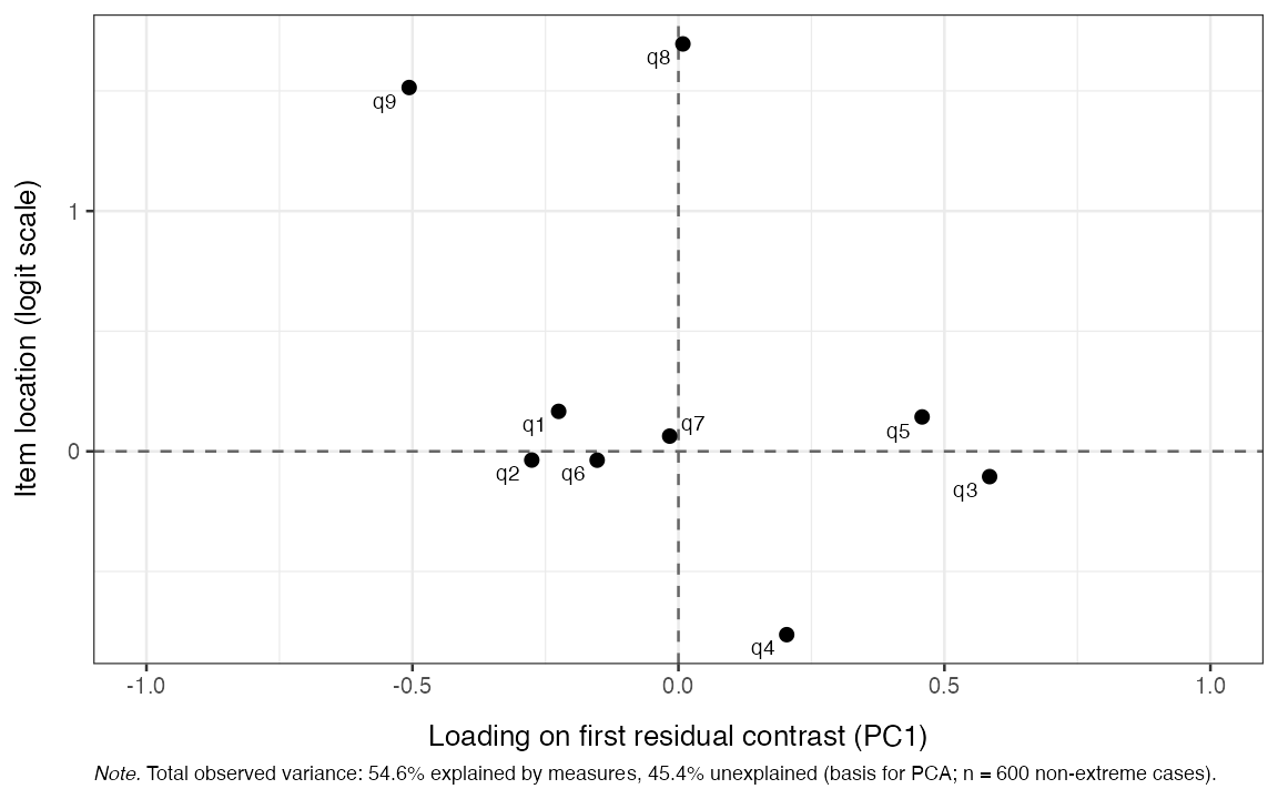

Figure 4. Standardized loadings on the first residual contrast

Martin-Löf test

This is a likelihood-ratio test of unidimensionality against an a priori specified multidimensional alternative. The p-value is obtained by parametric-bootstrap (Monte Carlo) sampling under the unidimensional null. A significant p-value constitutes strong evidence that items do not all measure one common latent variable. However, while a non-significant p-value indicates that data are consistent with one common latent variable across the partition, it is not to be considered proof of unidimensionality on its own.

In the use case demonstrated below, we have hypothesized that the five psychosomatic symptoms are a separate subscale from the other items. Looking at the PCA plot above, we can see tendencies of this clustering based on the loadings on the first residual contrast factor, with items 3-5 most clearly deviating from 1, 2, 6, and 9. Using the PCA plot to determine item partitioning for the M-L test is not recommended; see ?RMdimMartinLof for details and references.

mlof <- RMdimMartinLof(items, iterations = 100,
                       partition = list(
                         c("q1","q2","q6","q9"),
                         c("q3","q4","q5","q7","q8")
                       ),
                       seed = 4
)

mlof$p_value
#> [1] 0.00990099
mlof$wle_correlation
#>   subscale_a subscale_b         r ci_lower  ci_upper      p_value   n
#> 1          1          2 0.7174163 0.676203 0.7541533 5.994126e-96 600

The p-value rejects unidimensionality across the partition, while the subscale WLE correlation indicates the dimensions are strongly related. Note that the Monte Carlo p-value’s resolution is limited by the number of iterations: the attainable values are k/(B+1), so with B = 100 iterations the smallest possible p-value is 1/101 \approx 0.0099 (returned as mlof$p_value_floor). A p-value equal to that floor means that no simulated statistic reached the observed one and should be read as p < 0.01 — the true p-value may be much smaller. Use more iterations (e.g. 1000, floor \approx 0.001) when reporting results. The M-L test results can be further investigated using the diagnostic function RMdimMartinLofResiduals().

2. Local independence

Local independence (LD) can be assessed with multiple methods. Yen’s Q_3 statistic (Yen 1984) is the correlation between person-item standardized residuals for every item pair. Pair-wise Q_3 values above the simulation-based cutoff flag LD (Christensen et al. 2017).

q3_cut <- RMlocdepQ3Cutoff(items, iterations = 100, parallel = FALSE,
                           seed = 4)
q3_results <- RMlocdepQ3(items, cutoff = q3_cut)
q3_results$matrix

Dynamic cut-off: 0.031 (mean Q3 -0.109 + 0.14). Global simulation cutoff (99th pctl of max-mean Q3) from 100 iterations. Correlations exceeding the cut-off may indicate local dependence; see the per-pair table for detail. n = 600 respondents.
	q1	q2	q3	q4	q5	q6	q7	q8	above_cutoff
q1
q2	0.23								*
q3	-0.19	-0.19
q4	0	-0.03	0.08						*
q5	-0.2	-0.25	0.09	0					*
q6	-0.18	0.02	-0.15	-0.14	-0.12
q7	-0.13	-0.18	-0.2	-0.08	-0.13	-0.05
q8	-0.17	-0.3	-0.18	-0.16	-0.1	-0.18	0.08		*
q9	-0.12	0.06	-0.23	-0.31	-0.24	0.02	-0.19	-0.11	*

For a more powerful Q_3 test, one can use the simulated cutoffs object to plot the expected range of residual correlations for each item-pair and compare with the observed value. We’ll limit the output to the 6 item-pairs that deviate the most.

q3_plots <- RMlocdepQ3Plot(simfit = q3_cut, data = items, n_pairs = 6)
q3_plots$pairs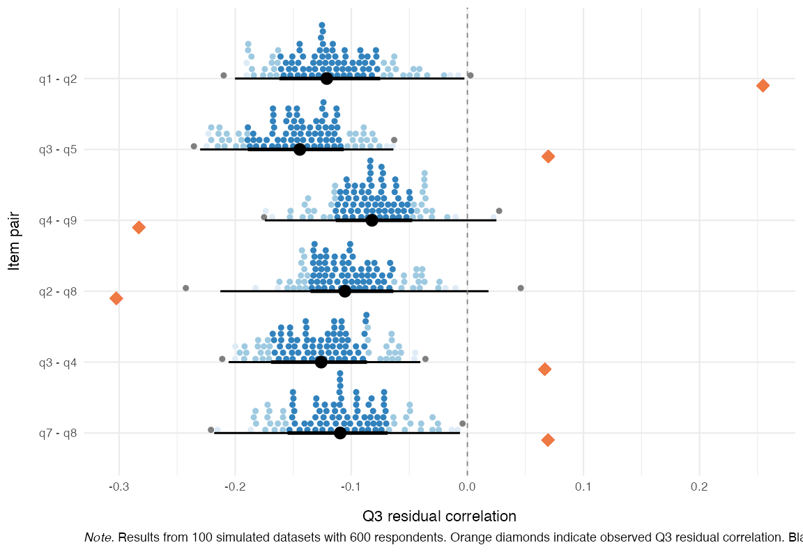

Figure 5. Observed and expected Q_3 residuals

Here we can see that the overfit item 2 does indeed have the strongest LD issues, primarily with item 1, but also with item 9. For analysis of multidimensionality, it can also be interesting to see which items have lower than expected residual correlations.

Partial gamma LD

A second perspective on LD is the partial gamma coefficient (Kreiner and Christensen 2004; Kreiner 2007) between observed item pairs, conditional on the rest-score. Note that this function evaluates both directions of LD, thus the output is two tables. We’ll restrict the output to the 6 item-pairs with largest LD deviations.

RMlocdepGamma(items, n_pairs = 6)

Partial gamma LD analysis. n = 600 respondents. Positive gamma indicates positive local dependence between items. Showing top 6 of 36 pairs by |gamma|. Direction 1: rest score = total - Item2.
Item 1	Item 2	Partial gamma	Adj. p-value (BH)	p-value sign.
q1	q2	0.531	0.000	***
q4	q9	-0.381	0.000	***
q2	q9	0.332	0.001	***
q2	q8	-0.323	0.001	***
q7	q8	0.303	0.001	***
q6	q9	0.287	0.009	**

Partial gamma LD analysis. n = 600 respondents. Positive gamma indicates positive local dependence between items. Showing top 6 of 36 pairs by |gamma|. Direction 2: rest score = total - Item2 (item pairs shown in the reverse order to direction 1).
Item 1	Item 2	Partial gamma	Adj. p-value (BH)	p-value sign.
q2	q1	0.577	0.000	***
q9	q4	-0.453	0.000	***
q8	q2	-0.415	0.000	***
q4	q3	0.361	0.000	***
q5	q3	0.303	0.000	***
q9	q2	0.291	0.007	**

You can also get simulation-based thresholds for partial gamma LD, using RMlocdepGammaCutoff(), which can be used with RMlocdepGamma() and also to plot the results with RMlocdepGammaPlot()

Item pairs flagged by both Q_3 and partial gamma are the strongest candidates for further inspection or possible item revision. Some argue for creating testlets by combining a locally dependent pair into a single polytomous super-item rather than eliminating one in an LD pair. I suggest looking closely at the item content before taking any action. Often, one will see very similarly worded items, where one item in an LD pair is clearly redundant. Another solution to LD can be the Graphical Loglinear Rasch Model by Kreiner and Christensen (Kreiner 2007), but that is beyond the scope of this vignette.

3. Ordered response category thresholds

For a polytomous item to function as intended, the thresholds separating adjacent response categories should be ordered: the threshold from “Not at all” to “Several days” should sit below the one from “Several days” to “More than half the days”, and so on.

A classical method to assess item response functions is to plot probability of response curves for each item and response category.

RMitemCatProb(items, category_labels = item_resp)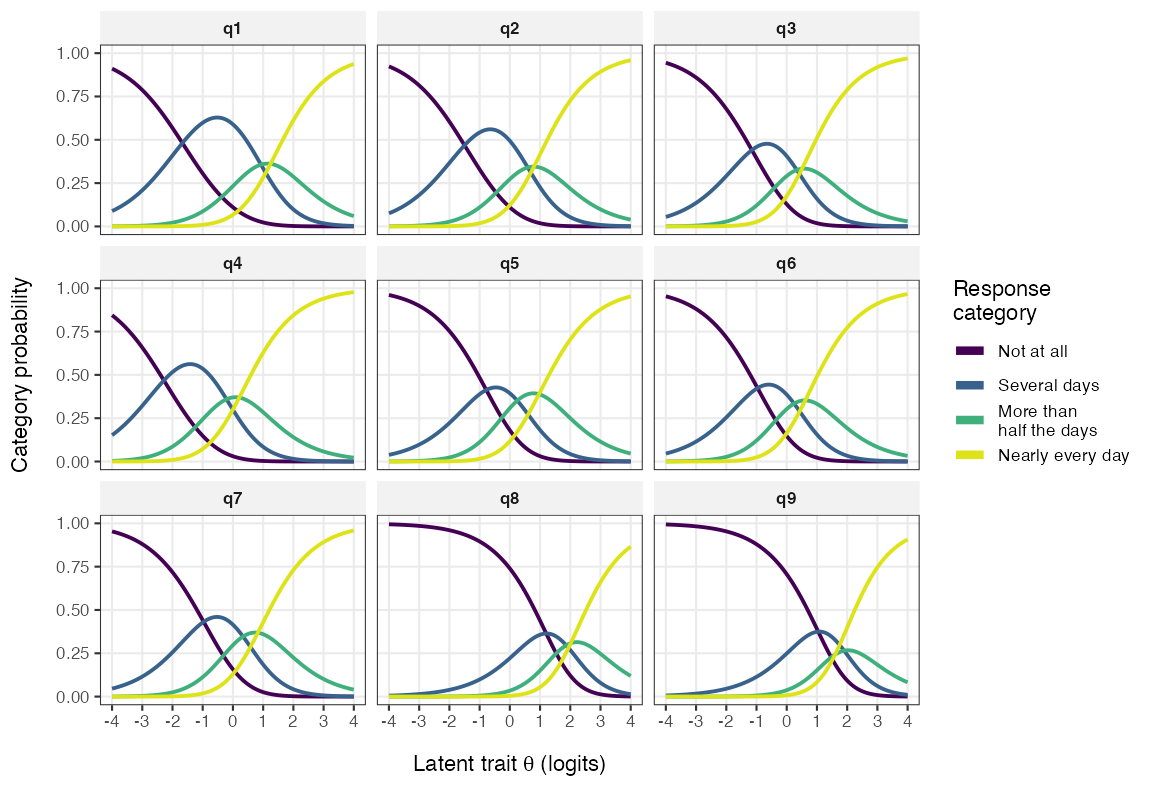

Figure 6. Item Probability Function curves

In the plot above, each category curve should be the most likely response at some part of the latent continuum (x axis). Item category thresholds are the points where two adjacent category lines cross each other (where they are both equally probable). In the plot above, we can see that the second highest category does not work well compared to other categories. It is disordered for item 9 and, as is perhaps clearer in the plot below, shows very small distances from the adjacent categories in most items (see T2 and T3 below, which are the lower and upper thresholds for “More than half the days”).

RMitemHierarchy() plots each item’s threshold locations on the latent scale, ordered by overall item difficulty. Disordered thresholds appear as overlapping or reversed segments and are a clear signal that the response categories are not being used in the intended order.

RMitemHierarchy(items, item_labels = item_desc)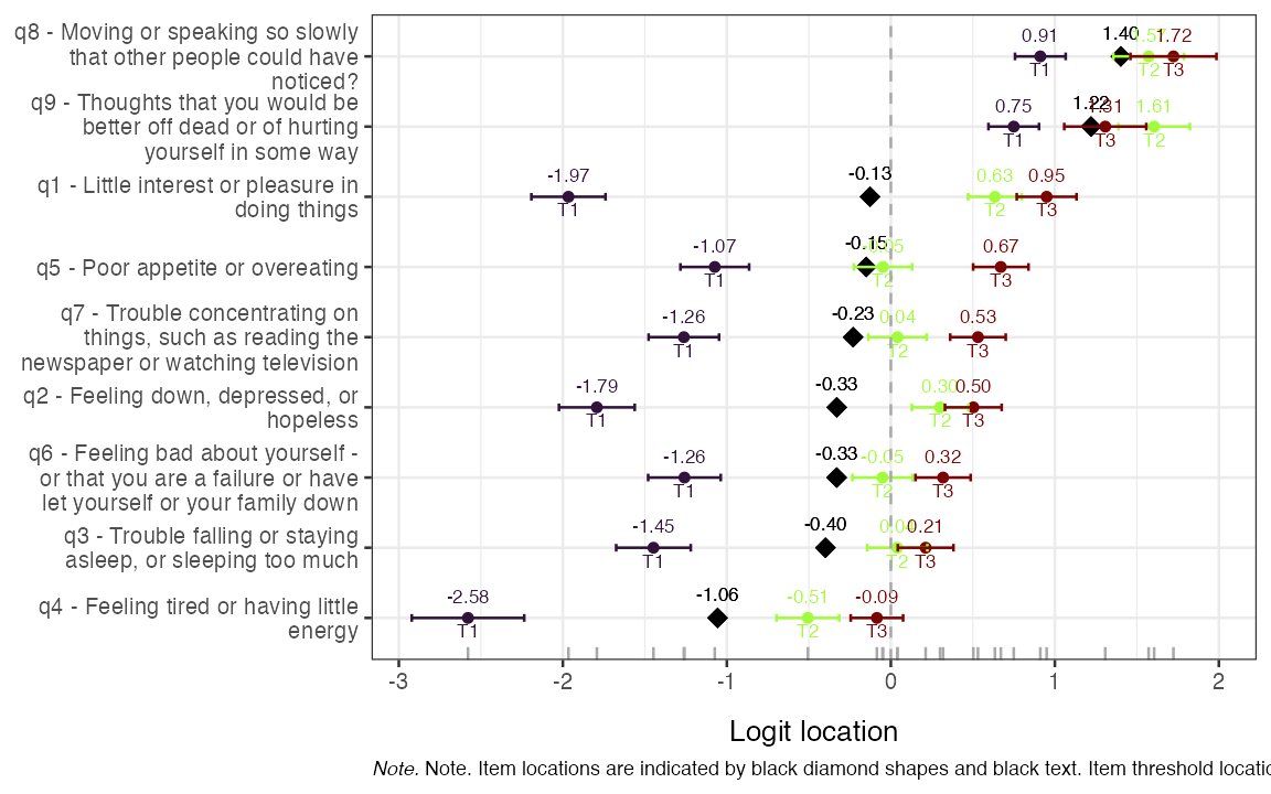

Figure 7. Item-hierarchy

4. Invariance / no DIF

We use three complementary DIF assessments. The Andersen likelihood-ratio test (LRT, Andersen 1973) partitions the sample by an external variable, refits the model in each subgroup, and compares item locations. The partial gamma approach (Kreiner 2007; Christensen et al. 2021) looks for an association between item responses and the external variable conditional on the rest-score, and the Rasch tree (below) searches for DIF across covariates without pre-specified groups. All are run on the gender variable, which has some missing values that are automatically dropped by the functions (noted in a console message and/or table/figure caption output).

First, it is important to review the response distribution when dividing the sample. If there are zero or low (below 8 or so) responses in a category, there may be issues with estimating the model parameters.

RMplotTile(items, category_labels = item_resp, group = phq9$gender)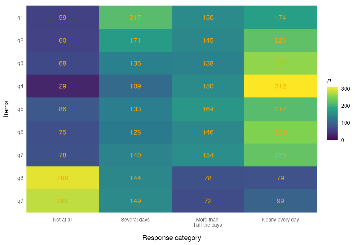

Figure 8. DIF grouped response distribution tile plot

Andersen LR-test

RMdifLR(items, dif_var = phq9$gender, level = "threshold", output = "ggplot")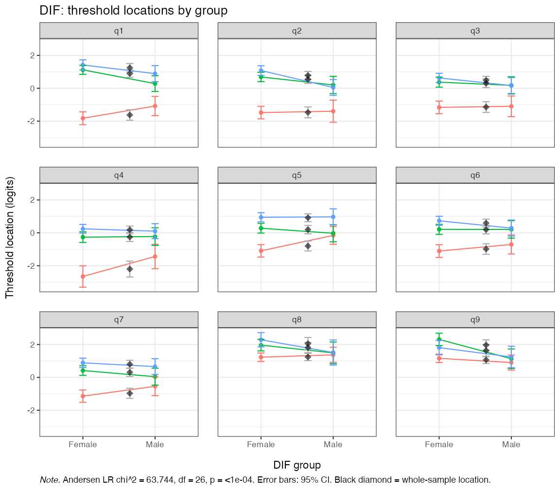

Figure 9. Andersen LR-test DIF locations by gender

The plot shows the item threshold locations estimated in each gender group with the corresponding confidence band. The global LR test is also reported in the plot caption, with a statistically significant test indicating problems with DIF between groups. However, this test is sensitive to sample size and number of items and should, like all global tests, be interpreted with care.

Partial-gamma DIF

This plot annotates each item with its partial-\gamma DIF coefficient and shows group differences within class intervals (respondents grouped by their total/latent score).

RMitemICCPlot(items, dif_var = phq9$gender, error_band = TRUE)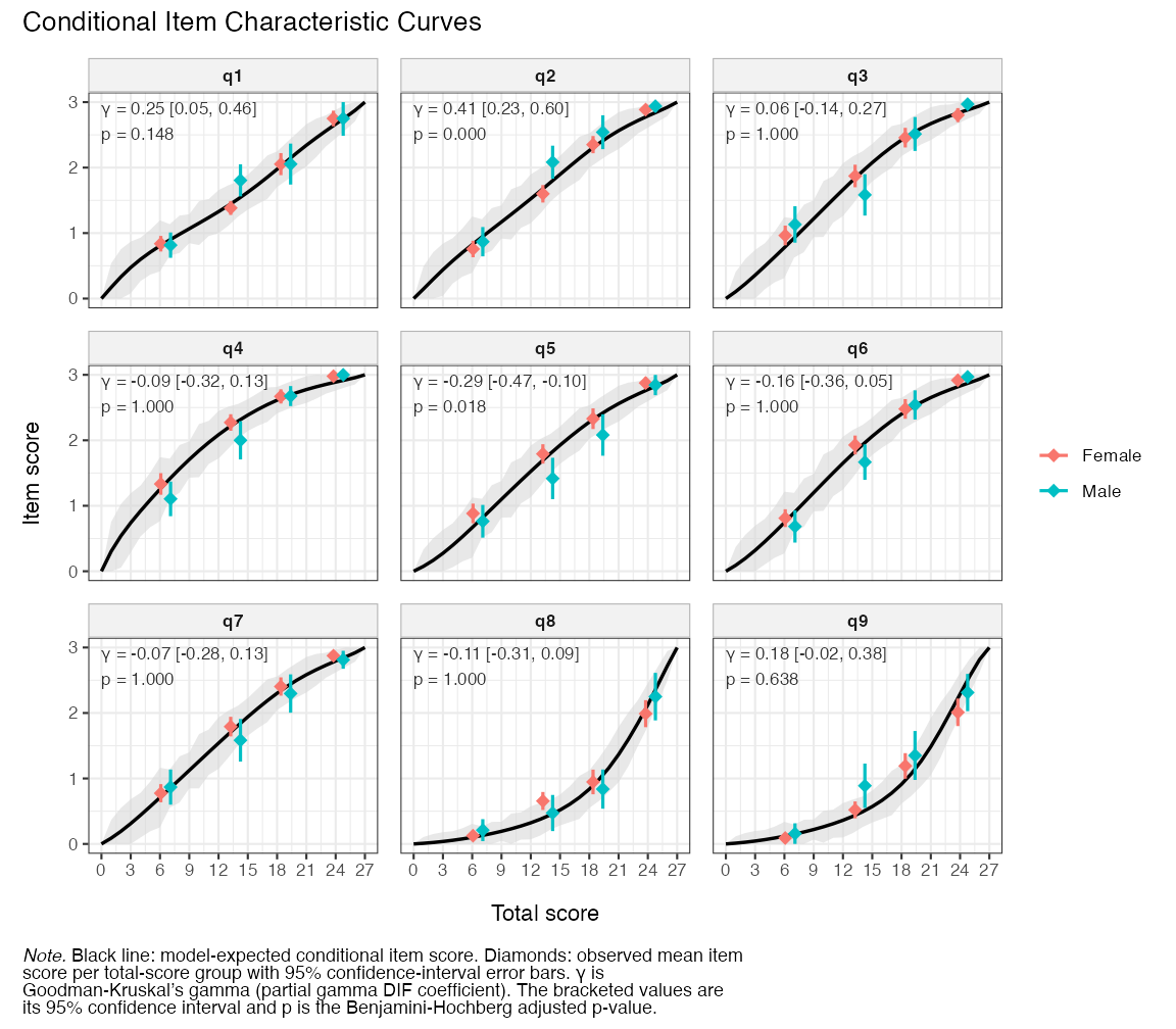

Figure 10. Partial Gamma DIF Conditional Item Characteristic Curves

To demonstrate the FWER-adjusted p-values, we’ll run the partial-\gamma DIF analysis with parametric bootstrap (only 100 here for rendering speed, which limits the reliability of the p-values).

difpg <- RMdifGammaCutoff(items, dif_var = phq9$gender, iterations = 100,
                          parallel = FALSE, seed = 5)
RMdifGamma(items, cutoff = difpg, dif_var = phq9$gender, p_value = TRUE)

Partial gamma DIF analysis. n = 569 of 600 respondents (complete cases). Two-sided bootstrap p-values from 100 iterations (replacing the asymptotic BH p-values); multiplicity correction: Westfall-Young step-down (FWER); flagged at padj < 0.05. p-values cannot be smaller than 1/(100+1) = 0.0099. Positive gamma indicates higher scores in higher DIF group levels.
Item	Partial gamma	SE	Lower CI	Upper CI	Gamma low	Gamma high	p	p (adj)	Flagged
q1	0.251	0.104	0.046	0.456	-0.218	0.260	0.0198	0.0693	FALSE
q2	0.411	0.094	0.227	0.595	-0.241	0.205	0.0099	0.0099	TRUE
q3	0.064	0.103	-0.138	0.266	-0.248	0.252	0.4752	0.6238	FALSE
q4	-0.092	0.114	-0.315	0.131	-0.177	0.236	0.2574	0.5941	FALSE
q5	-0.286	0.092	-0.467	-0.104	-0.212	0.190	0.0099	0.0099	TRUE
q6	-0.155	0.105	-0.361	0.050	-0.206	0.180	0.1782	0.5545	FALSE
q7	-0.075	0.102	-0.275	0.126	-0.219	0.214	0.4356	0.6238	FALSE
q8	-0.112	0.102	-0.311	0.088	-0.181	0.241	0.2574	0.5941	FALSE
q9	0.180	0.100	-0.015	0.376	-0.226	0.206	0.0495	0.2178	FALSE

Rasch tree (model-based recursive partitioning)

The DIF methods above compare groups that we specify in advance. The Rasch tree approach (Strobl et al. 2015) instead searches for DIF: the model is fitted to the full sample, covariates are tested for parameter instability, and whenever instability is detected the sample is split at the covariate value that maximizes it. The procedure then repeats within each subgroup, so several useful things come for free. Continuous covariates such as age need no arbitrary pre-categorization — the optimal cutpoint is estimated from the data. Interactions are handled naturally, since later splits are conditional on earlier ones (e.g. a gender split appearing only among older respondents). And if no instability is found, the tree simply does not split.

Statistically significant splits are not necessarily important splits, particularly in large samples. RMdifTree() therefore pairs the tree with an effect-size classification for every item at every split (Henninger et al. 2025): the Mantel-Haenszel odds ratio on the Delta scale developed at the Educational Testing Service (ETS) for dichotomous data, or the partial gamma coefficient for polytomous data, classified into the ETS categories A (negligible), B (slight to moderate), and C (moderate to large) (Holland and Thayer 1986; Zwick 2012). For partial gamma the B/C boundaries are the familiar 0.21 / 0.31 used by RMdifGamma(), so the two functions read on the same scale. Note that these boundaries are conventions carried over from large-scale educational testing, not values calibrated to your sample and items — in contrast to the simulation-based cutoffs used elsewhere in this package — so the A/B/C labels are best read as a rough magnitude guide rather than a calibrated test.

RMdifTree(items, covariates = phq9$gender)

Node 1 – gender: Female vs Male (n left = 426, n right = 143)

Partial Credit Tree (9 items). n = 569 of 600 respondents (complete DIF covariates). Effect size: partial gamma (B/C thresholds = 0.21 / 0.31). alpha = 0.05. Flagged (Class B or C): 3 / 9 (item x split combinations). **Bold** rows are flagged.
Item	EffectSize	SE	Class	Flagged
q1	0.2508	0.1045	B	yes
q2	0.4113	0.0939	C	yes
q3	0.0637	0.1031	A	no
q4	-0.0923	0.1137	A	no
q5	-0.2857	0.0925	B	yes
q6	-0.1553	0.1048	A	no
q7	-0.0747	0.1023	A	no
q8	-0.1118	0.1018	A	no
q9	0.1804	0.0999	A	no

The tree splits on gender, and the effect sizes match what the partial gamma analysis showed above: q2 is classified as C and q1 and q5 as B, while the remaining items are negligible (A). With a single binary covariate the tree reduces to the familiar two-group comparison — its advantages appear when you supply several covariates at once (covariates = phq9[, c("gender", "age")]), where it tests all of them, picks split points for continuous ones, and uncovers interactions.

Three options are worth knowing about: purification = “iterative” recomputes effect sizes while excluding already-flagged items from the matching score; stability = TRUE refits the tree on resamples to report how often each covariate is selected and where the cutpoints land — a guard against overinterpreting a single sample’s tree structure; and output = “plot” draws the tree with per-node item parameters.

Next step

Since we found issues with item misfit, local dependence, and gender DIF, these need to be addressed before the scale is used for measurement. Notably, item 2 recurs across all three criteria — overfit, the strongest local dependence (with item 1), and the largest gender DIF — making it the natural first candidate for closer inspection. The recommended approach is iterative: remove a single item (for instance, an underfit item, or one item from an LD pair after reviewing item content), then re-run the full set of analyses, since fit indications for the remaining items change with every removal. When the sample is large enough, it is good practice to set aside a random holdout subsample before the analysis, so that the final item set can be confirmed in data that played no part in the item-reduction decisions.

The following sections are primarily of interest once an acceptable item set has been established; here we continue with all nine items for demonstration purposes.

Targeting

A targeting plot summarizes how well the item-threshold distribution matches the distribution of person locations on the latent scale — a Wright-map style display.

RMtargeting(items)
#> Error in `seq.default()`:
#> ! 'to' must be a finite number

Reliability

RMreliability() reports four reliability metrics: person separation reliability (PSI); Relative Measurement Uncertainty (RMU) estimate derived from posterior person-location uncertainty using plausible values; Cronbach’s alpha; and marginal reliability. PSI, alpha and marginal can use bootstrap for confidence intervals. All reliability metrics range from 0 to 1, with higher values indicating better separation/precision.

RMreliability(items, draws = 200, rmu_iter = 20, parallel = FALSE,
              seed = 6)

Reliability for 9 items, n = 600 respondents. PSI is the WLE-based separation reliability and excludes min/max scoring respondents.
Metric	Estimate	Lower (95% HDCI)	Upper (95% HDCI)	Notes
Cronbach’s alpha	0.886	NA	NA	no bootstrap
PSI	0.838	NA	NA	no bootstrap
Marginal	0.862	NA	NA	no bootstrap
RMU (WLE)	0.881	0.867	0.895	200 PVs, 20 RMU iterations

Item and person parameters

Item (threshold) locations can be easily summarized in wide or long format, with or without SEs.

RMitemParameters(items, format = "wide")

Item thresholds via CML (Andrich thresholds, logit scale). SE shown. n = 600 respondents.
item	t1	t2	t3	location	se_t1	se_t2	se_t3
q1	-1.966	0.634	0.950	-0.127	0.165	0.115	0.124
q2	-1.793	0.300	0.503	-0.330	0.168	0.122	0.118
q3	-1.447	0.039	0.212	-0.399	0.166	0.130	0.116
q4	-2.578	-0.506	-0.085	-1.056	0.250	0.136	0.109
q5	-1.074	-0.048	0.671	-0.150	0.153	0.125	0.115
q6	-1.259	-0.051	0.318	-0.330	0.161	0.130	0.114
q7	-1.262	0.041	0.531	-0.230	0.157	0.125	0.115
q8	0.912	1.572	1.723	1.402	0.110	0.151	0.180
q9	0.749	1.605	1.307	1.221	0.110	0.153	0.172

Person parameters are also sometimes referred to as thetas, latent scores, or person locations. By default, Warm’s weighted likelihood estimation (WLE) is used for minimal bias. The function exports one value and SE for each individual, below reduced to only print the first 10 rows of the dataframe. Note that all table outputs in easyRasch2 can be output as dataframes instead, if so desired. The option output = "file" makes it easy to export estimated latent scores for each respondent to a CSV file.

ppar <- RMpersonParameters(items, output = "dataframe")
head(ppar, 10)
#>         theta       sem sum_score n_answered extreme
#> 1   2.2760818 0.6184838        25          9   FALSE
#> 2  -0.9997531 0.4658741         7          9   FALSE
#> 3   1.1406643 0.4262412        20          9   FALSE
#> 4   0.3379335 0.3959994        15          9   FALSE
#> 5   3.6996335 1.3248428        27          9    TRUE
#> 6   1.1406643 0.4262412        20          9   FALSE
#> 7  -0.6129841 0.4288279         9          9   FALSE
#> 8   0.9701100 0.4155331        19          9   FALSE
#> 9   0.6465516 0.4019393        17          9   FALSE
#> 10 -3.2339486 0.9216600         1          9   FALSE

Ordinal-to-interval transformation

For converting ordinal sum-scores to interval-scaled person-location estimates with associated standard errors, use RMscoreSE().

RMscoreSE(items, output = "ggplot")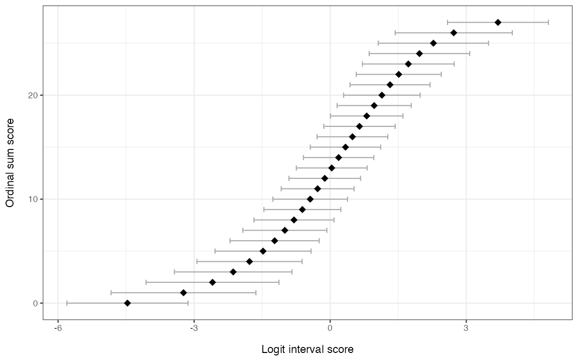

Figure 12. Sum-score to WLE conversion with 95% CIs

RMscoreSE(items)

Person locations via Warm’s WLE (CML item parameters). n = 600 respondents.
Ordinal sum score	Logit score	Logit std.error
0	-4.469	1.536
1	-3.234	0.922
2	-2.594	0.737
3	-2.138	0.638
4	-1.779	0.574
5	-1.480	0.528
6	-1.224	0.493
7	-1.000	0.466
8	-0.798	0.445
9	-0.613	0.429
10	-0.440	0.417
11	-0.277	0.408
12	-0.119	0.401
13	0.034	0.397
14	0.186	0.396
15	0.338	0.396
16	0.491	0.398
17	0.647	0.402
18	0.806	0.408
19	0.970	0.416
20	1.141	0.426
21	1.320	0.441
22	1.512	0.462
23	1.723	0.492
24	1.968	0.539
25	2.276	0.618
26	2.724	0.778
27	3.700	1.325

RMscoreSE() also has an option for EAP scores (expected a posteriori).

Person fit

Conditional person infit/outfit MSQ and the \ell_z statistic are implemented, with Monte-Carlo resampling for p-values.

pfit <- RMpersonFit(items, iterations = 100, output = "ggplot", seed = 7)
pfit$lz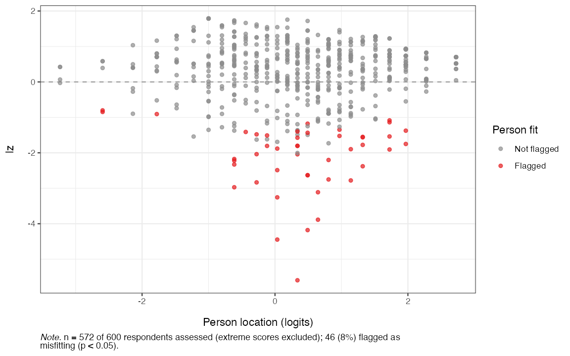

Figure 13. Person fit with the lz statistic

Where to next

Each RM*() function is documented with its own ?function reference page including a worked example.
The simulation-based cutoffs used above (RM*Cutoff()) can be parallelised on multiple CPU cores via the mirai package; see the relevant help pages.
- For a progress bar on time-consuming simulations, add verbose = TRUE to the function call. This should not be used when rendering Quarto/Rmd files.

References

Andersen, Erling B. 1973. “A Goodness of Fit Test for the Rasch Model.” Psychometrika 38 (1): 123–40. https://doi.org/10.1007/BF02291180.

Chou, Yeh-Tai, and Wen-Chung Wang. 2010. “Checking Dimensionality in Item Response Models With Principal Component Analysis on Standardized Residuals.” Educational and Psychological Measurement 70 (5): 717–31. https://doi.org/10.1177/0013164410379322.

Christensen, Karl Bang, Jonathan D. Comins, Michael R. Krogsgaard, et al. 2021. “Psychometric Validation of PROM Instruments.” Scandinavian Journal of Medicine & Science in Sports 31 (6): 1225–38. https://doi.org/10.1111/sms.13908.

Christensen, Karl Bang, and Svend Kreiner. 2007. “A Monte Carlo Approach to Unidimensionality Testing in Polytomous Rasch Models.” Applied Psychological Measurement 31 (1): 20–30. https://doi.org/10.1177/0146621605286204.

Christensen, Karl Bang, Guido Makransky, and Mike Horton. 2017. “Critical Values for Yen’s Q3: Identification of Local Dependence in the Rasch Model Using Residual Correlations.” Applied Psychological Measurement 41 (3): 178–94. https://doi.org/10.1177/0146621616677520.

Henninger, Mirka, Jan Radek, Rudolf Debelak, and Carolin Strobl. 2025. “Partial Credit Trees Meet the Partial Gamma Coefficient for Quantifying DIF and DSF in Polytomous Items.” Behaviormetrika 52: 221–57. https://doi.org/10.1007/s41237-024-00252-3.

Holland, Paul W., and Dorothy T. Thayer. 1986. “Differential Item Functioning and the Mantel-Haenszel Procedure.” ETS Research Report Series 1986 (2): i–24. https://doi.org/10.1002/j.2330-8516.1986.tb00186.x.

Johansson, Magnus. 2025. “Detecting Item Misfit in Rasch Models.” Educational Methods & Psychometrics 3 (18). https://doi.org/10.61186/emp.2025.5.

Kreiner, Svend. 2007. “Validity and Objectivity: Reflections on the Role and Nature of Rasch Models.” Nordic Psychology 59 (3): 268–98. https://doi.org/10.1027/1901-2276.59.3.268.

Kreiner, Svend. 2011. “A Note on Item–Restscore Association in Rasch Models.” Applied Psychological Measurement 35 (7): 557–61. https://doi.org/10.1177/0146621611410227.

Kreiner, Svend, and Karl Bang Christensen. 2004. “Analysis of Local Dependence and Multidimensionality in Graphical Loglinear Rasch Models.” Communications in Statistics - Theory and Methods 33 (6): 1239–76. https://doi.org/10.1081/STA-120030148.

Kroenke, Kurt, Robert L. Spitzer, and Janet B. W. Williams. 2001. “The PHQ-9: Validity of a Brief Depression Severity Measure.” Journal of General Internal Medicine 16 (9): 606–13. https://doi.org/10.1046/j.1525-1497.2001.016009606.x.

Müller, Marianne. 2020. “Item Fit Statistics for Rasch Analysis: Can We Trust Them?” Journal of Statistical Distributions and Applications 7 (1): 5. https://doi.org/10.1186/s40488-020-00108-7.

Strobl, Carolin, Julia Kopf, and Achim Zeileis. 2015. “Rasch Trees: A New Method for Detecting Differential Item Functioning in the Rasch Model.” Psychometrika 80 (2): 289–316. https://doi.org/10.1007/s11336-013-9388-3.

Yen, Wendy M. 1984. “Effects of Local Item Dependence on the Fit and Equating Performance of the Three-Parameter Logistic Model.” Applied Psychological Measurement 8 (2): 125–45. https://doi.org/10.1177/014662168400800201.

Zwick, Rebecca. 2012. “A Review of ETS Differential Item Functioning Assessment Procedures: Flagging Rules, Minimum Sample Size Requirements, and Criterion Refinement.” ETS Research Report Series 2012 (1): i–30. https://doi.org/10.1002/j.2333-8504.2012.tb02290.x.