Item Category Probability Curves

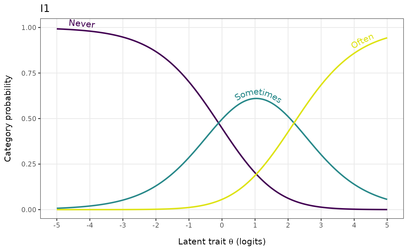
Plots model-implied response-category probability curves for each item as a function of the latent trait $\theta$. Polytomous items are fitted with the Partial Credit Model via eRm::PCM(); dichotomous items are fitted with the Rasch model via eRm::RM(). Each item gets its own facet panel, with one curve per response category coloured from low to high using the viridis palette. Comparable in scope to eRm::plotICC() and mirt's trace plots, with a ggplot2 / viridis output and optional descriptive labels for items and categories.

Usage

RMitemCatProb(
  data,
  item_labels = NULL,
  category_labels = NULL,
  theta_range = NULL,
  n_points = 200L,
  viridis_option = "D",
  viridis_end = 0.95,
  facet_ncol = NULL,
  label_wrap = 25L,
  line_width = 0.9,
  font = "sans",
  output = c("ggplot", "dataframe"),
  label_curves = c("legend", "path"),
  item = NULL,
  text_size = 4
)

Arguments

data: A data.frame or matrix of item responses. Items must be scored starting at 0 (non-negative integers). Missing values (NA) are allowed — the model fit handles them.
item_labels: Optional character vector of descriptive item labels (facet strip titles). Must be the same length as ncol(data). If NULL (the default), column names are used.
category_labels: Optional character vector of labels for the response categories (legend). Must be the same length as the number of categories spanning from 0 to the maximum observed value. If NULL (the default), numeric category values are used.
theta_range: Numeric length 2. Range of the latent trait $\theta$ (logits) plotted along the x-axis. When NULL (default) the range is c(-4, 4) for label_curves = "legend" and a wider c(-5, 5) for label_curves = "path" — the wider range gives geomtextpath more horizontal room to place per-curve labels at their peaks. Pass an explicit c(lo, hi) to override.
n_points: Integer. Number of evenly-spaced $\theta$ values at which the curves are evaluated. Default 200L.
viridis_option: Character. Viridis palette identifier. One of "A" through "H". Default "D" (viridis green).
viridis_end: Numeric in (0, 1]. Upper end of the viridis palette range; lower values keep the palette inside its mid-tones (avoids the very bright yellow at 1.0). Default 0.95.
facet_ncol: Optional integer. Number of columns in the facet layout. Default NULL (ggplot2::facet_wrap() auto-layout).
label_wrap: Integer. Characters per line for facet-strip label wrapping. Default 25L.
line_width: Numeric. Line width for the probability curves. Default 0.9.
font: Character. Font family for all text. Default "sans".
output: Character. Either "ggplot" (default) for a ggplot object, or "dataframe" for the underlying long-format probability table.
label_curves: Character. How response categories are identified. "legend" (default) draws lines and a separate colour legend with one swatch per category — the standard multi-item presentation. "path" uses geomtextpath::geom_textpath() to write each category's label along its own curve (a la classic IRT trace plots) and suppresses the legend; valid for a single item at a time because narrow facets do not give path labels enough horizontal room to render legibly. The model is still fit on the full multi-item data (PCM thresholds require multi-item input for CML estimation); the item argument then selects which item's curves to plot. Requires the optional geomtextpath package.
item: Character or integer. Used only when label_curves = "path". Either an item name (matching a column in data) or a column index, identifying which item's category curves to plot. Required for path mode.
text_size: Numeric. Used only when label_curves = "path". Size of the path labels in mm. Default 4.

Value

If output = "ggplot": a ggplot2::ggplot object, one facet per item.
If output = "dataframe": a long-format data.frame with columns Item (factor in column order), Category (integer), and Theta, Probability (numeric), one row per item × category × theta gridpoint.

Details

For each polytomous item i with response categories $0, 1, \ldots, K_i$ and threshold parameters $\delta_{i,1}, \ldots, \delta_{i,K_i}$ from eRm::thresholds(), the PCM category probability is

$$P(X_i = k \mid \theta) = \frac{\exp(\sum_{j=1}^{k} (\theta - \delta_{i,j}))}{\sum_{k'=0}^{K_i} \exp(\sum_{j=1}^{k'} (\theta - \delta_{i,j}))},$$

with the empty sum (when $k = 0$) taken as zero. For dichotomous items the function fits a Rasch model and treats the item difficulty $\delta_i = -\beta_i$ as the single threshold, recovering the standard two-category logistic ICC.

The colour mapping uses scale_color_viridis_c() against the integer category value, so the natural ordering of response categories is preserved visually — low categories at one end of the palette, high categories at the other. When category_labels is provided, the legend uses those labels (e.g., "Never" / "Sometimes" / "Often") while the colour mapping stays on the integer category value.

Items with fewer response categories than the maximum (e.g., an otherwise four-category scale with one three-category item) contribute only the categories they actually have to their own facet — the y-axis still spans $[0, 1]$.

Examples

# \donttest{
if (requireNamespace("eRm", quietly = TRUE) &&
    requireNamespace("ggplot2", quietly = TRUE)) {
  data(pcmdat2, package = "eRm")

  # Default plot
  RMitemCatProb(pcmdat2)

  # Custom item and category labels
  RMitemCatProb(
    pcmdat2,
    item_labels     = c("Mood", "Sleep", "Appetite", "Energy"),
    category_labels = c("Never", "Sometimes", "Often")
  )

  # Underlying probability data
  df <- RMitemCatProb(pcmdat2, output = "dataframe")
  head(df)

  # Single-item plot with labels written along each curve
  # (classic IRT trace-plot style). Model is still fit on all four
  # items; `item` picks which one to plot.
  if (requireNamespace("geomtextpath", quietly = TRUE)) {
    RMitemCatProb(
      pcmdat2,
      category_labels = c("Never", "Sometimes", "Often"),
      label_curves    = "path",
      item            = "I1"
    )
  }
}

# }

Usage

Arguments

Value

Details

See also

Examples