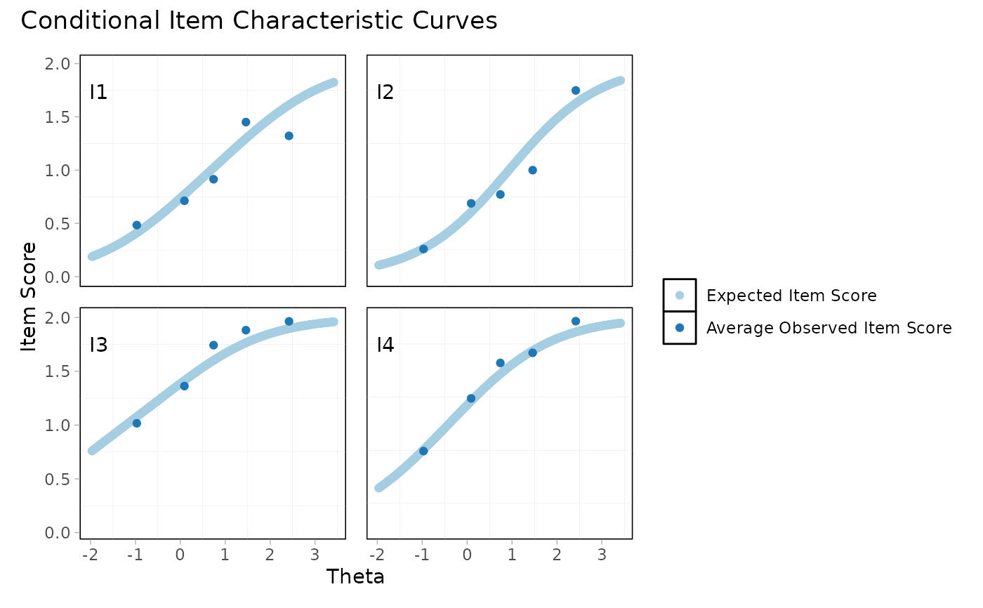
Conditional Item Characteristic Curves

Faceted panel of Conditional Item Characteristic Curves (cICCs), one per item. Each panel shows the model-expected conditional item score \(E[X_i \mid R = r]\) against the total score \(r\), together with the average observed item score within class intervals of the total score and their confidence intervals. When a dif_var is supplied, observed averages are computed separately per group, turning each panel into a visual DIF check, and the partial-gamma DIF magnitude is reported per item.

Usage

RMitemICCPlot(
  data,
  dif_var = NULL,
  method = c("quantile", "width", "score", "manual", "cut"),
  class_intervals = 4,
  score_breaks = NULL,
  ci = TRUE,
  error_band = FALSE,
  conf_level = 0.95,
  min_n = 8L,
  items = NULL,
  output = c("patchwork", "list")
)

Arguments

data: A data.frame or matrix of item responses (non-negative integers, 0-based). One column per item, one row per person.
dif_var: Optional vector of length nrow(data) (factor or coercible to factor) defining a DIF grouping variable. When supplied, observed averages are shown separately per group and the partial-gamma DIF coefficient (iarm::partgam_DIF(), as in RMdifGamma()) is annotated per panel. Default NULL (no DIF).
method: How the observed means are grouped along the total score (see Class intervals in Details). One of "quantile" (default): class_intervals groups of approximately equal numbers of respondents; "width": class_intervals equal-width intervals over the observed total-score range; "score": every observed total score is its own group; or "manual": groups defined by score_breaks. "cut" is accepted as a legacy alias for "quantile".
class_intervals: Integer >= 2. Number of class intervals for method = "quantile" and method = "width". Default 4. Ignored (without an error) by method = "score" and method = "manual".
score_breaks: Integer vector for method = "manual": the total scores at which a new group starts, in increasing order. For example, score_breaks = c(3, 6, 8) on a 0-9 scale defines the groups 0-2, 3-5, 6-7, and 8-9 (the endpoints are added automatically). Serves the same purpose as lower.groups in RASCHplot's CICCplot(), without the leading zero. Default NULL.
ci: Logical. Draw confidence intervals (error bars) on the observed class-interval means. Default TRUE.
error_band: Logical. Add a shaded band around the model-expected curve: the model's interval for the observed mean at each total score, \(E \pm z \sqrt{\mathrm{Var}/n_r}\) (n_r = number of respondents at that total score), as in RASCHplot's CICCplot. Complementary to ci, not a replacement – see Details. Default FALSE.
conf_level: Numeric in (0, 1). Confidence level for the observed error bars and the model band. Default 0.95.
min_n: Integer. A group-by-interval cell needs at least this many respondents to contribute an observed point + CI; sparser cells are skipped. Default 8 (the package's per-cell stability floor).
items: Optional character or integer vector selecting which items to plot. The model is always fitted on all items; only the rendering is filtered. Default NULL (all items).
output: One of "patchwork" (default) – composite patchwork figure – or "list" – a named list of per-item ggplot objects.

Value

Either a patchwork/ggplot composite (default) or a named list of per-item ggplot objects (output = "list"). In DIF mode the per-item partial-gamma table is attached as attr(., "dif_gamma").

Details

The model curve and its conditional variance come from the shared CML engine (CML item thresholds via psychotools and the exact conditional distribution of each item score given the total score, via elementary symmetric functions). The conditional-ICC approach follows Buchardt, Christensen & Jensen (2023) and their RASCHplot package; the implementation here is native to easyRasch2's CML/WLE engine.

Conditioning. The expected curve is the exact conditional expectation of the item score given the total score (it accounts for the item being part of the total), not a marginal ICC.

Class intervals. Following Buchardt et al. (2023), the empirical item means can be shown for each value of the total score or for each value of the grouped total score; all grouping happens on the total-score scale (never on an estimated latent score). Four grouping rules are available. method = "quantile" (the default) splits the observed total scores into class_intervals bins of approximately equal numbers of respondents, using common boundaries so DIF groups share the x-axis – the same approach as iarm::ICCplot()'s class intervals (Hmisc::cut2(g = ...)). method = "width" instead splits the observed score range into class_intervals intervals of equal width, which reads naturally on the score axis but can leave sparse intervals (pruned by min_n). method = "score" uses every observed total score as its own group – the maximal-resolution display, sensible for short scales, with min_n pruning thinly-populated scores. method = "manual" places the group boundaries exactly where you say via score_breaks (RASCHplot's lower.groups concept). Each bin contributes one observed point at its mean total score. If the score distribution is too sparse to form class_intervals distinct bins, the quantile and width methods fall back to score-level points.

Confidence intervals. Observed error bars use the normal approximation \(\bar{x}_l \pm z \sqrt{\mathrm{var}(x_l) / n_l}\) within each (group, interval) cell, clamped to the item's score range; cells with fewer than min_n respondents are dropped. In DIF mode this makes sparse group differences visibly uncertain rather than over-interpreted.

The model band (error_band). The shaded band is drawn around the model-expected curve at \(E_{ri} \pm z \sqrt{V_{ri}/n_r}\), where \(E_{ri}\) and \(V_{ri}\) are the exact conditional mean and variance of the item score given total score \(r\) (model quantities), and \(n_r\) is the observed number of respondents at that total score. If the Rasch model is true, this is where the empirical mean item score at total score \(r\) should fall, given how many people actually sit at that score; an observed diamond outside the band is localized graphical misfit. The band is deliberately the standard error of the mean (\(\sqrt{V/n_r}\)), not the far wider individual-response SD band, which would flag nothing. Its width therefore tracks the data: narrow where many respondents sit (a strict test), wide in sparse score regions (a lenient one), with gaps where \(n_r = 0\) and collapsing to the curve at the deterministic extremes (total score 0 and the maximum). It is complementary to, not a replacement for, the ci error bars: the band is the model-implied uncertainty of the observed mean per raw score; the error bars are the sample-based uncertainty of the observed group means.

DIF magnitude. The annotated partial gamma (Bjorner et al., 1998) is the association between the item score and the group conditional on the rest score – a non-parametric effect size, complementary to the total-score-conditional visual. It is the same statistic as RMdifGamma().

References

Buchardt, A.-S., Christensen, K. B., & Jensen, S. N. (2023). Visualizing Rasch item fit using conditional item characteristic curves in R. Psychological Test and Assessment Modeling, 65(2), 206-219.

Andersen, E. B. (1995). Polytomous Rasch models and their estimation. In G. H. Fischer & I. W. Molenaar (Eds.), Rasch Models: Foundations, Recent Developments, and Applications (pp. 271-291). Springer. (Conditional expectation of item scores given the total score; formula 15.22.)

Bjorner, J. B., Kreiner, S., Ware, J. E., Damsgaard, M. T., & Bech, P. (1998). Differential item functioning in the Danish translation of the SF-36. Journal of Clinical Epidemiology, 51(11), 1189-1202.

Examples

# \donttest{
if (requireNamespace("ggplot2", quietly = TRUE) &&
    requireNamespace("patchwork", quietly = TRUE) &&
    requireNamespace("iarm", quietly = TRUE)) {
  set.seed(42)
  sim_data <- as.data.frame(
    matrix(sample(0:2, 200 * 4, replace = TRUE), nrow = 200, ncol = 4)
  )
  colnames(sim_data) <- paste0("Item", 1:4)

  # Default: quantile groups (~equal numbers of respondents per group)
  RMitemICCPlot(sim_data)

  # Equal-width intervals on the total-score scale, with the model band
  RMitemICCPlot(sim_data, method = "width", error_band = TRUE)

  # Every total score as its own group (short scales)
  RMitemICCPlot(sim_data, method = "score")

  # Manual grouping: new groups start at total scores 3, 5, and 7
  RMitemICCPlot(sim_data, method = "manual", score_breaks = c(3, 5, 7))
}

# }