---
title: "easyRasch vignette"
subtitle: "R package for Rasch analysis"
author:
name: 'Magnus Johansson'
affiliation: 'Karolinska Institutet'
affiliation-url: 'https://ki.se/en/people/magnus-johansson-3'
orcid: '0000-0003-1669-592X'
date: last-modified
google-scholar: true
citation: true
website:
open-graph:
image: "/RaschRvign_files/figure-html/unnamed-chunk-34-1.png"
execute:
cache: true
warning: false
message: false
bibliography:
- references.bib
- grateful-refs.bib
csl: apa.csl
editor_options:
chunk_output_type: console
---
This is an introduction to using the [`easyRasch` R package](https://pgmj.github.io/easyRasch/). A changelog for package updates is available [here](https://pgmj.github.io/easyRasch/news/index.html).
I have also created a package for Bayesian Rasch models, based on the
[`brms`](https://paulbuerkner.com/brms/) package and several of the functions showcased in this vignette.
You can find [`easyRaschBayes`](https://pgmj.github.io/easyRaschBayes/index.html) on
[CRAN](https://cloud.r-project.org/web/packages/easyRaschBayes/index.html).
If you find this package and/or vignette helpful, consider buying me a coffee?
<a href="https://www.buymeacoffee.com/pgmj" target="_blank"><img src="https://cdn.buymeacoffee.com/buttons/default-orange.png" alt="Buy Me A Coffee" height="41" width="174"></a>
::: {.callout-important icon="true"}
## Note
**MacOS 26.1+ known issue**: Upgrade package `vcdExtra` to version 0.9.3, or add this code to your easyRasch scripts before loading package `iarm`: `options(rgl.useNULL = TRUE)`.
More details available here: <https://stackoverflow.com/a/66127391>
:::
::: {.callout-note icon="true"}
## Note
This package was previously known as `RISEkbmRasch`.
:::
Details on package installation are available at the [package GitHub page](https://pgmj.github.io/easyRasch).
If you are new to Rasch Measurement Theory, you may find this intro presentation useful:
<https://pgmj.github.io/RaschIRTlecture/slides.html>
This vignette will walk through a sample analysis using an open dataset with polytomous questionnaire data. This will include some data wrangling to structure the item data and itemlabels, then provide examples of the different functions. The full source code of this document can be found either [in this repository](https://github.com/pgmj/pgmj.github.io/blob/main/raschrvignette/RaschRvign.qmd) or by clicking on **\</\> CODE** at the top of this page. You should be able to use the source code "as is" and reproduce this document locally, as long as you have the required packages installed. This page and this website are built using the open source publishing tool [Quarto](https://www.quarto.org).
One of the aims with this package is to simplify reproducible psychometric analysis to shed light on the measurement properties of a scale, questionnaire or test. In line with others [@kreiner_validity_2007;@christensen_rasch_2013], I propose that the basic psychometric criteria for a set of items to be used as a measure of a latent variable are:
- Unidimensionality (for each subscale, if there are multiple)
- Local independence of items
- Ordered response categories
- Invariance (differential item functioning)
And that we should also report information regarding:
- Targeting
- Measurement uncertainties (reliability)
- Person fit
We'll include several ways to investigate these measurement properties, using Rasch Measurement Theory. There are also functions in the package less directly related to the criteria above, that will be demonstrated in this vignette.
Please note that this is just a sample analysis to showcase the R package. It is not intended as a "best practice" psychometric analysis example.
You can skip ahead to the Rasch analysis part in @sec-rasch if you are eager to look at the package output :)
There is a separate GitHub repository containing a template R-project to simplify using the `easyRasch` package when conducting a reproducible Rasch analysis in R: <https://github.com/pgmj/RISEraschTemplate>
## Getting started
Since the package is intended for use with Quarto, this vignette has also been created with Quarto. A "template" .qmd file [is available](https://github.com/pgmj/RISEraschTemplate/blob/main/analysis.qmd) that can be useful to have handy for copy&paste when running a new analysis. You can also download a complete copy of the Quarto/R code to produce this document [here](https://github.com/pgmj/pgmj.github.io/blob/main/raschrvignette/RaschRvign.qmd).
Loading the `easyRasch` package will automatically load all the packages it depends on. However, it could be desirable to explicitly load all packages used, to simplify the automatic creation of citations for them, using the `grateful` package (see @sec-grateful).
```{r}
library(easyRasch) # devtools::install_github("pgmj/easyRasch", dependencies = TRUE)
library(grateful)
library(ggrepel)
library(car)
library(kableExtra)
library(readxl)
library(tidyverse)
library(eRm)
library(iarm)
library(mirt)
library(psych)
library(ggplot2)
library(psychotree)
library(matrixStats)
library(reshape)
library(knitr)
library(patchwork)
library(formattable)
library(glue)
library(foreach)

### some commands exist in multiple packages, here we define preferred ones that are frequently used
select <- dplyr::select
count <- dplyr::count
recode <- car::recode
rename <- dplyr::rename
```
::: {.callout-note icon="true"}
## Note
Quarto automatically adds links to R packages and functions throughout this document. However, this feature only works properly for packages available on [CRAN](https://cran.r-project.org/). Since the `easyRasch` package is not on CRAN the links related to functions starting with **RI** will not work.
:::
### Loading data
We will use data from a recent paper investigating the "initial elevation effect" [@anvari2022], and focus on the 10 negative items from the PANAS. The data is available at the OSF website.
```{r}
df.all <- read_csv("https://osf.io/download/6fbr5/")
# if you have issues with the link, please try downloading manually using the same URL as above
# and read the file from your local drive.

# subset items and demographic variables
df <- df.all %>%
  select(starts_with("PANASD2_1"),
         starts_with("PANASD2_20"),
         age,Sex,Group) %>%
  select(!PANASD2_10_Active) %>%
  select(!PANASD2_1_Attentive)
```
The `glimpse()` function provides a quick overview of our dataframe.
```{r}
glimpse(df)
```
We have `r nrow(df)` rows, ie. respondents. All variables except Sex and Group are of class `dbl`, which means they are numeric and can have decimals. Integer (numeric with no decimals) would also be fine for our purposes. The two demographic variables currently of class `chr` (character) will need to be converted to factors (`fct`), and we will do that later on.
(If you import a dataset where item variables are of class character, you will need to recode to numeric.)
### Itemlabels
Then we set up the itemlabels dataframe. This could also be done using the free [LibreOffice Calc](https://www.libreoffice.org/download/download-libreoffice/) or MS Excel. Just make sure the file has the same structure, with two variables named `itemnr` and `item` that contain the item variable names and item description. The item variable names have to match the variable names in the item dataframe.
```{r}
itemlabels <- df %>%
  select(starts_with("PAN")) %>%
  names() %>%
  as_tibble() %>%
  separate(value, c(NA, "item"), sep ="_[0-9][0-9]_") %>%
  mutate(itemnr = paste0("PANAS_",c(11:20)), .before = "item")
```
The `itemlabels` dataframe looks like this.
```{r}
itemlabels
```
### Demographics
Variables for invariance tests such as Differential Item Functioning (DIF) need to be separated into vectors (ideally as factors with specified levels and labels) with the same length as the number of rows in the dataset. This means that any kind of removal of respondents/rows with missing data needs to be done before separating the DIF variables.
First, we'll have a look at the class of our variables.
```{r}
df %>%
  select(Sex,age,Group) %>%
  glimpse()
```
`Sex` and `Group` are class character, while `age` is numeric. Below are the response categories represented in data.
```{r}
table(df$Sex)
```
Since there are only 5 respondents using labels that are not Female or Male (too few for meaningful statistical analysis), we will remove them to have a complete dataset for all variables in this example.
```{r}
df <- df %>%
  filter(Sex %in% c("Female","Male")) # filtering to only include those with Sex being either Female or Male.
```
Let's make the variable a factor (instead of class "character"), since that will be helpful in our later analyses.
```{r}
df$Sex <- factor(df$Sex)
```
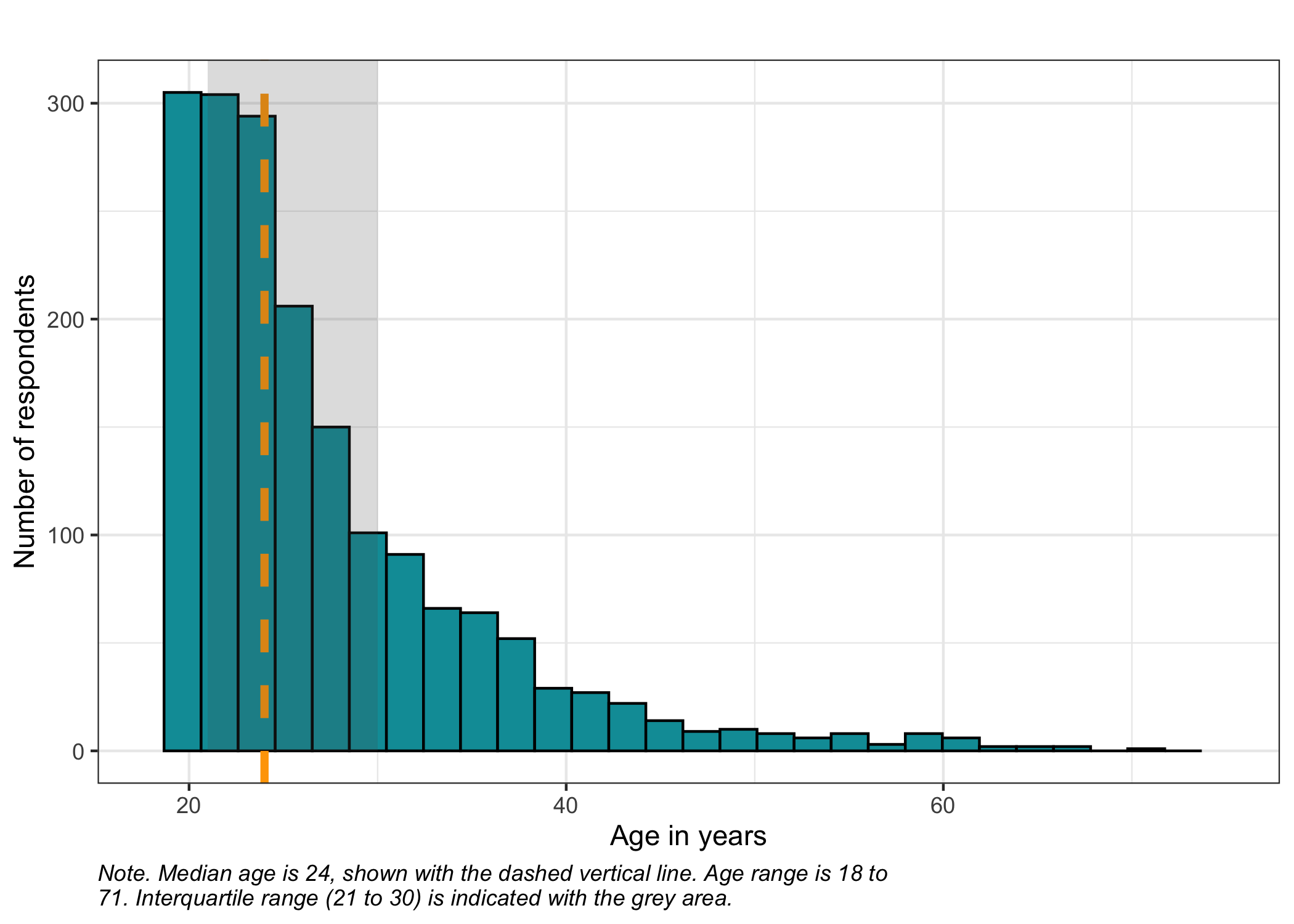
Sometimes age is provided in categories, but here we have a numeric variable with age in years. Let's have a quick look at the age distribution using a histogram, and get some summary statistics.
```{r}
summary(df$age)
```
```{r}
### simpler version of the ggplot below using base R function hist()
# hist(df$age, col = "#009ca6")
# abline(v = median(age, na.rm = TRUE))
#
# df %>%
#   summarise(Mean = round(mean(age, na.rm = T),1),
#             StDev = round(sd(age, na.rm = T),1)
#             )

ggplot(df) +
  geom_histogram(aes(x = age),
                 fill = "#009ca6",
                 col = "black") +
  # add the average as a vertical line
  geom_vline(xintercept = median(df$age),
             linewidth = 1.5,
             linetype = 2,
             col = "orange") +
  # add a light grey field indicating the standard deviation
  annotate("rect", ymin = 0, ymax = Inf,
           xmin = summary(df$age)[2],
           xmax = summary(df$age)[5],
           alpha = .2) +
  labs(title = "",
       x = "Age in years",
       y = "Number of respondents",
       caption = str_wrap(glue("Note. Median age is {round(median(df$age, na.rm = T),1)}, shown with the dashed vertical line. Age range is {min(df$age)} to {max(df$age)}. Interquartile range ({summary(df$age)[2]} to {summary(df$age)[5]}) is indicated with the grey area.")
       )) +
  scale_x_continuous(limits = c(18,75)) +
  theme_bw() +
  theme(plot.caption = element_text(hjust = 0, face = "italic"))
```
Since the distribution of the age variable is clearly not following a gaussian (normal) distribution, the median seems like a better option than the mean.
There is also a grouping variable which needs to be converted to a factor.
```{r}
df$Group <- factor(df$Group)
```
Now our demographic data has been checked, and we need to move it to a separate dataframe from the item data.
```{r}
dif <- df %>%
  select(Sex,age,Group) %>%
  rename(Age = age) # just for consistency

df <- df %>%
  select(!c(Sex,age,Group))
```
To create a "Table 1" containing participant demographic information, the `tbl_summary()` function from the `gtsummary` package is really handy to get a nice table.
```{r}
gtsummary::tbl_summary(dif)
```
With only item data remaining in the `df` dataframe, we can easily rename the items in the item dataframe and make sure that they match the `itemlabels` variable `itemnr`. It will be useful to have short item labels to get less clutter in the tables and figures during analysis.
```{r}
names(df) <- itemlabels$itemnr
```
Now we are all set for the psychometric analysis!
## Descriptives
Let's familiarize ourselves with the data before diving into the analysis.
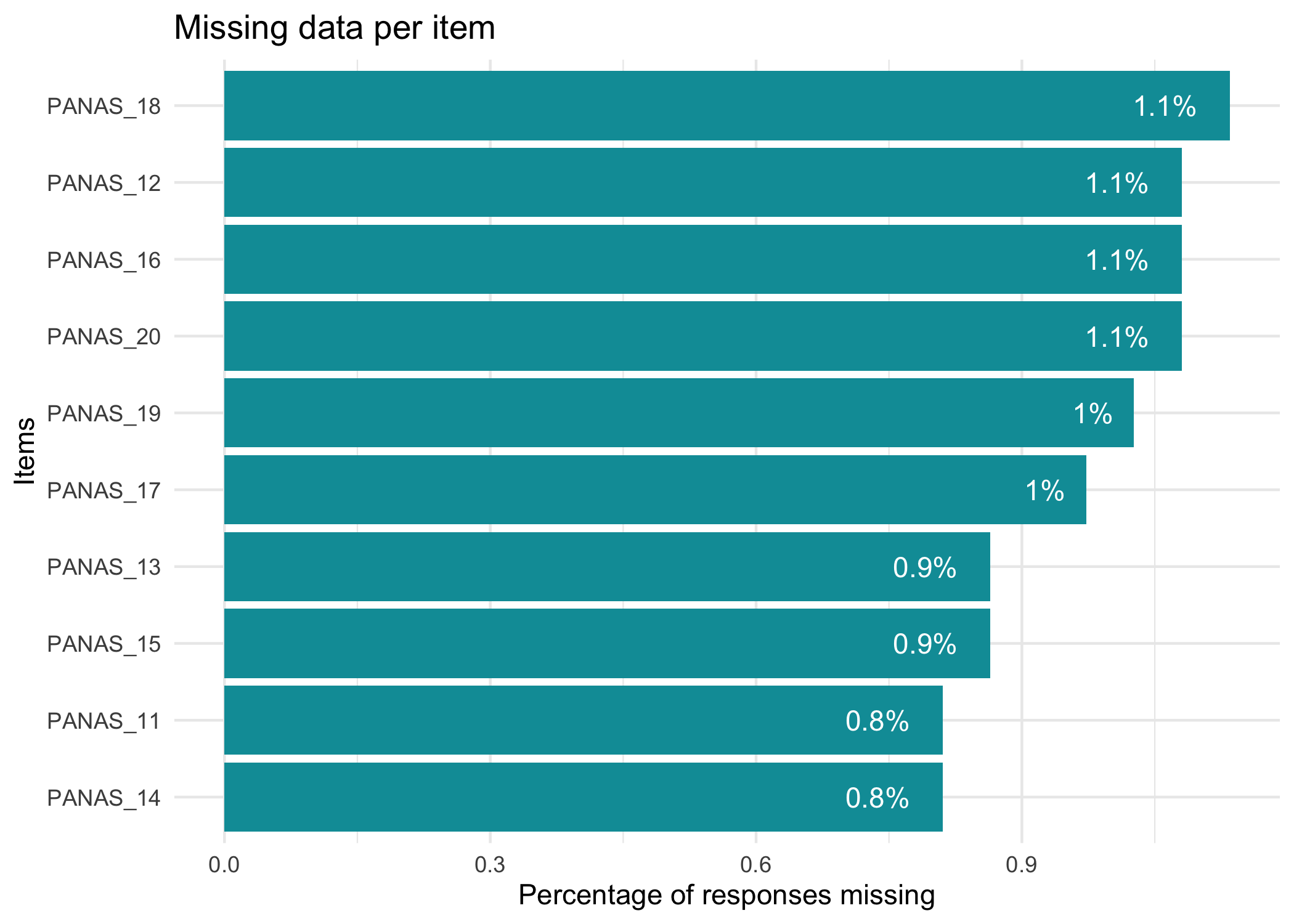
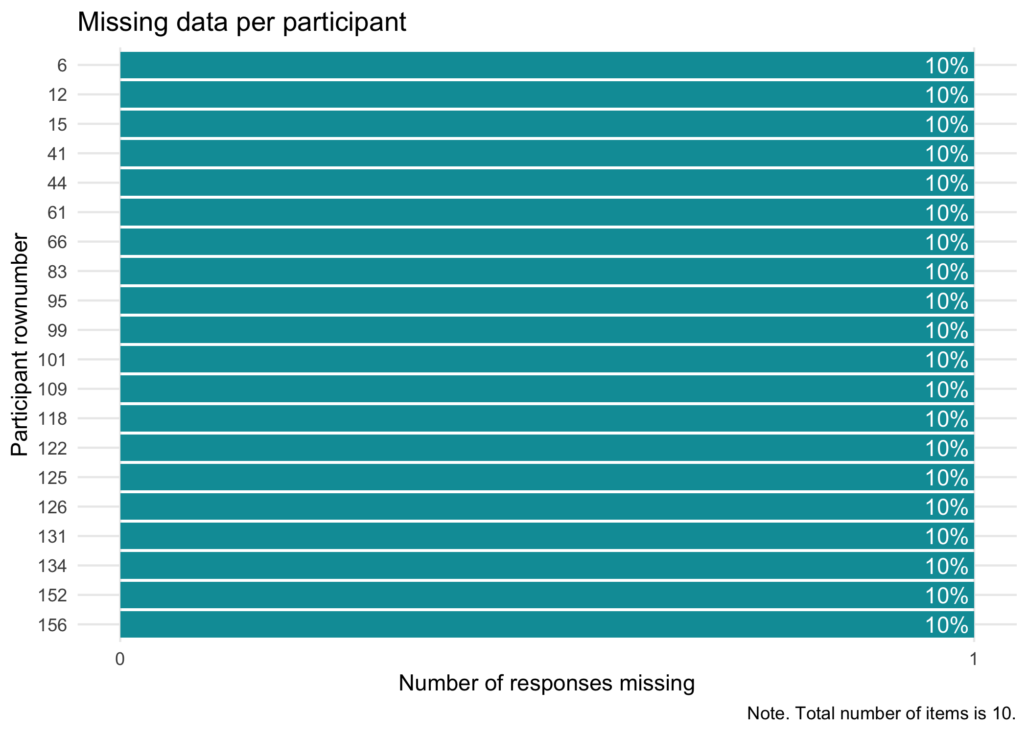
### Missing data
First, we visualize the proportion of missing data on item level.
```{r}
RImissing(df)
```
No missing data in this dataset. If we had missing data, we could also use `RImissingP()` to look at which respondents have missing data and how much. Just to show what the output of these functions looks like, we'll use `mice::ampute()` to temporarily remove 10% of data.
```{r}
RImissing(mice::ampute(df, prop = 0.1)$amp)
RImissingP(mice::ampute(df, prop = 0.1)$amp, N = 20)
```
### Overall responses
This provides us with an overall picture of the data distribution. As a bonus, any oddities/mistakes in recoding the item data from categories to numbers will be clearly visible.
```{r}
RIallresp(df)
```
Most R packages for Rasch analysis require the lowest response category to be coded as zero, which makes it necessary for us to recode our data, from the range of 1-5 to 0-4.
```{r}
df <- df %>%
  mutate(across(everything(), ~ .x - 1))

# always check that your recoding worked as intended.
RIallresp(df)
```
#### Floor/ceiling effects
We can also look at the raw distribution of ordinal sum scores. The `RIrawdist()` function is a bit crude, since it requires responses in all response categories to accurately calculate max and min scores.
```{r}
RIrawdist(df)
```
There is a floor effect with 11.8% of participants responding in the lowest category for all items.
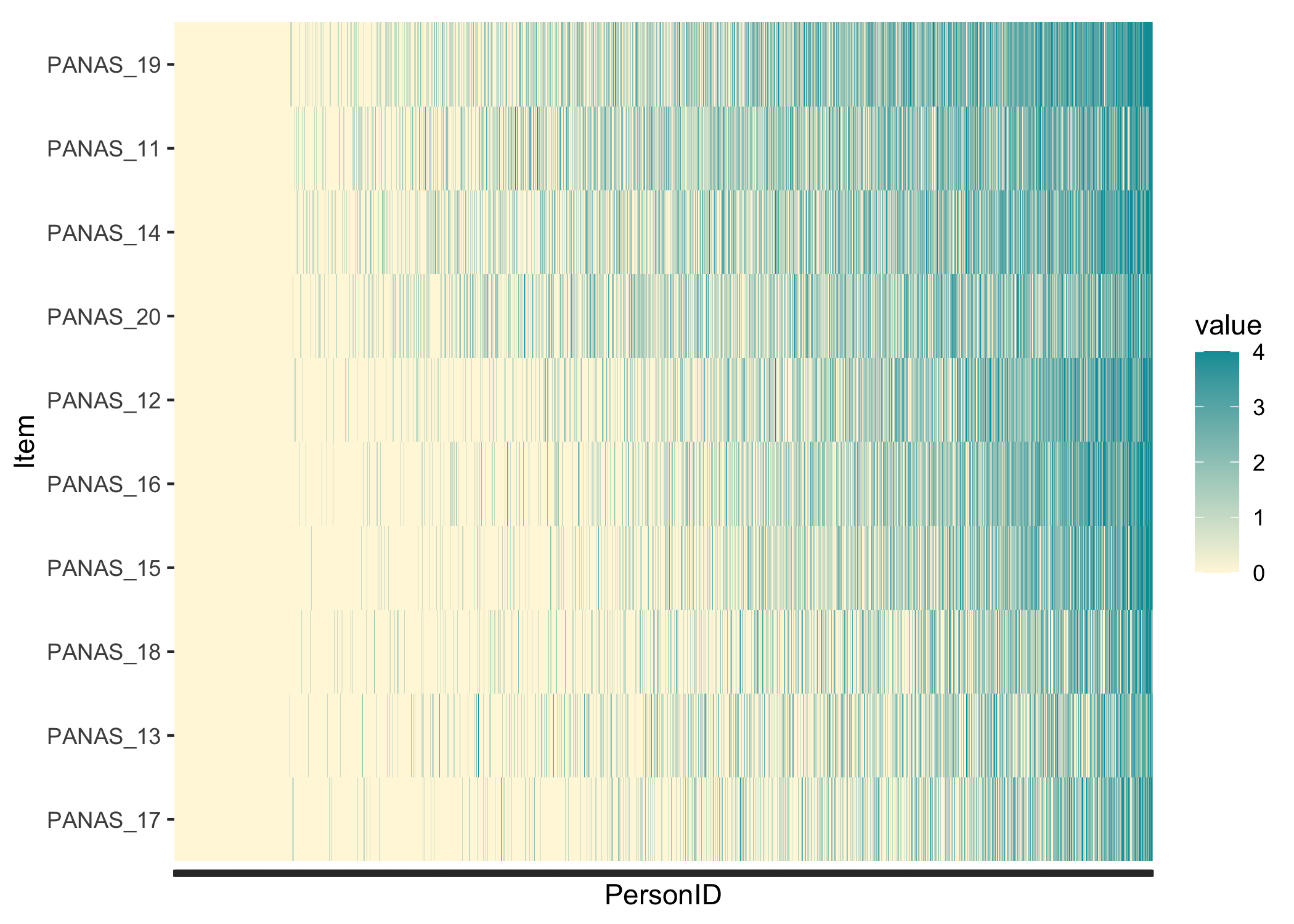
#### Guttman structure
While not really necessary, it can be interesting to see whether the response patterns follow a Guttman-like structure. Items and persons are sorted based on lower-\>higher responses, and we should see the color move from yellow in the lower left corner to blue in the upper right corner.
```{r}
RIheatmap(df) +
  theme(axis.text.x = element_blank())
```
In this data, we see the floor effect on the left, with 11.8% of respondents all yellow, and a rather weak Guttman structure. This could also be due to a low variation in item locations/difficulties. Since we have a very large sample I added a `theme()` option to remove the x-axis text, which would anyway just be a blur of the `r nrow(df)` respondent row numbers. Each thin vertical slice in the figure is one respondent.
### Item level descriptives
There are many ways to look at the item level data, and we'll get them all together in the tab-panel below. The `RItileplot()` is probably most informative, since it provides the number of responses in each response category for each item. It is usually recommended to have at least \~10 responses in each category for psychometric analysis, no matter which methodology is used.
Kudos to [Solomon Kurz](https://solomonkurz.netlify.app/blog/2021-05-11-yes-you-can-fit-an-exploratory-factor-analysis-with-lavaan/) for providing the idea and code on which the tile plot function is built!
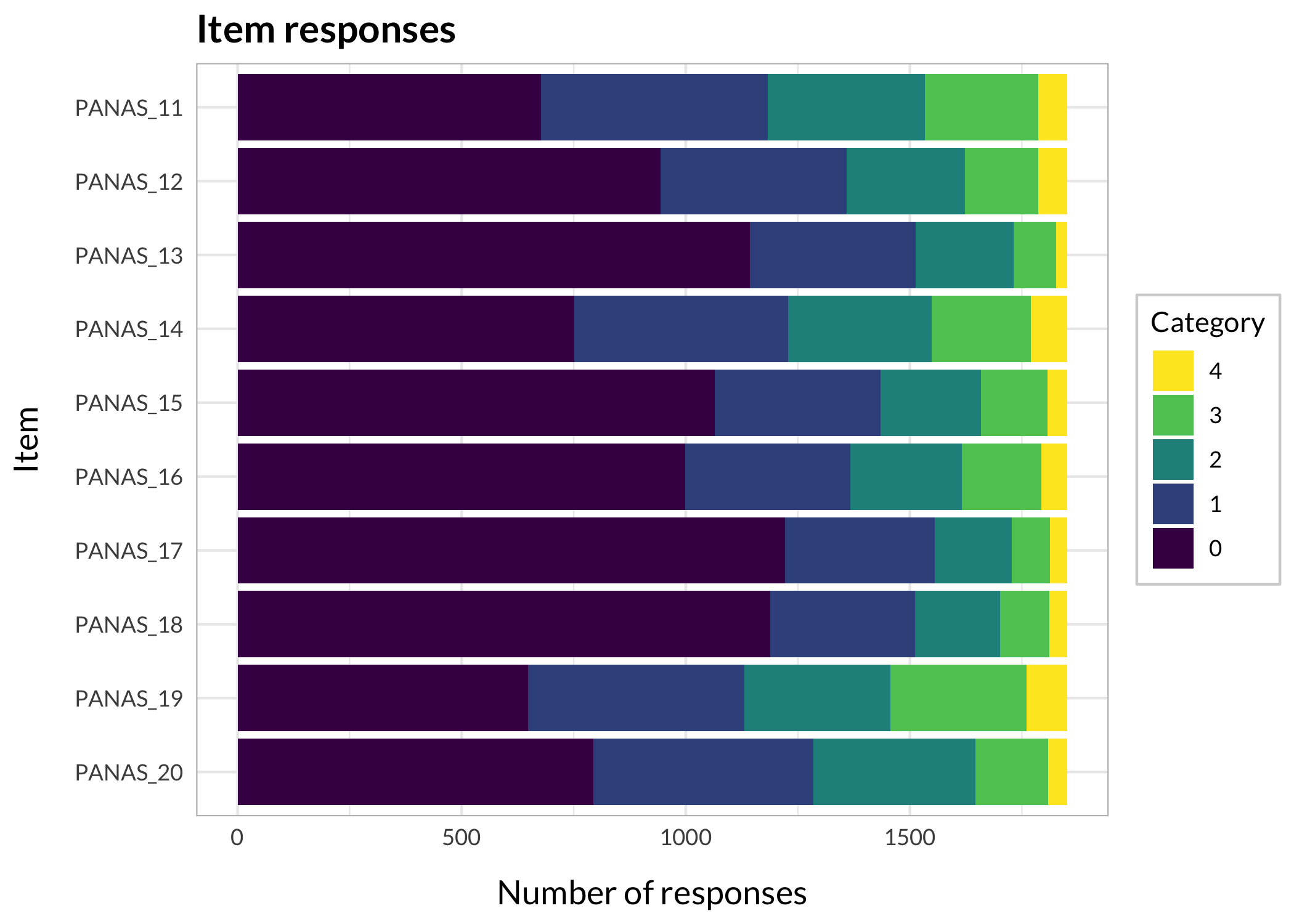
Most people will be familiar with the barplot, and this is probably most intuitive to understand the response distribution within each item. However, if there are many items it will take a while to review, and does not provide the same overview as a tileplot or stacked bars.
```{r}
#| column: margin
#| code-fold: true
#| echo: fenced
# This code chunk creates a small table in the margin beside the panel-tabset output below, showing all items currently in the df dataframe.
# The Quarto code chunk option "#| column: margin" is necessary for the layout to work as intended.
RIlistItemsMargin(df, fontsize = 13)
```
::: panel-tabset
#### Tile plot
```{r}
RItileplot(df)
```
While response patterns are skewed for all items, there are more than 10 responses in each category for all items which is helpful for the analysis.
#### Stacked bars
```{r}
RIbarstack(df) +
  theme_minimal() + # theming is optional, see section 11 for more on this
  theme_rise()
```
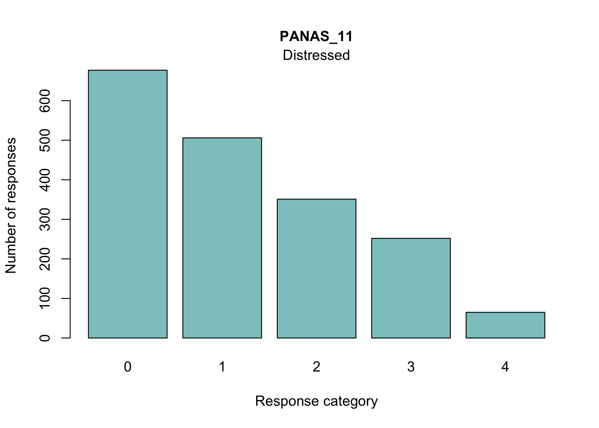
#### Barplots
```{r}
#| fig-height: 9
RIitemcols(df)
```
:::
## Rasch analysis 1 {#sec-rasch}
The eRm package and Conditional Maximum Likelihood (CML) estimation will be used primarily, with the Partial Credit Model since this is polytomous data. For more information about different estimation methods, see [@robitzsch_comprehensive_2021].
This is also where the basic psychometric aspects are good to recall.
- Unidimensionality
- Local independence
- Ordering of response categories
- Invariance
- Targeting
- Measurement uncertainties (reliability)
We will begin by looking at unidimensionality, response categories, and targeting in parallel below. For unidimensionality, we are mostly interested in item fit and residual correlations, as well as PCA of residuals and loadings on the first residual contrast. At the same time, disordered response categories can influence item fit to some extent (and vice versa), and knowledge about targeting can be useful if it is necessary to remove items due to residual correlations.
When unidimensionality and response categories are found to work adequately, we will move on to invariance testing (Differential Item Functioning, DIF). It should be noted that DIF should be evaluated in parallel with all other psychometric aspects, but since it is a more complex issue it is kept in a separate section in this vignette (as is person fit). Finally, when/if invariance/DIF also looks acceptable, we can investigate reliability/measurement uncertainties.
Since our sample is quite large (n > 800), the sample size sensitive tests (item fit and item-restscore) that are likely to produce problematic false positive rates [@johansson_detecting_2025] will use a randomly selected smaller sample of n = 500 as examples. When analyzing large datasets, item-restscore bootstrap is recommended as the primary method of assessing item fit to the Rasch model. **The use of one smaller subsample in this vignette is only for demonstration purposes, it is not a recommended method of analysis for large datasets.**
```{r}
df500 <- df %>%
  slice_sample(n = 500)
```
::: {.callout-note}
In the tabset-panel below, each tab contains explanatory text, which is sometimes a bit lengthy. Remember to **scroll back up and click on all tabs**.
:::
```{r}
#| column: margin
#| echo: false
RIlistItemsMargin(df, fontsize = 13)
```
::: panel-tabset
### Conditional item fit
```{r}
simfit1 <- RIgetfit(df500, iterations = 400, cpu = 8) # save simulation output to object `simfit1`
RIitemfit(df500, simfit1)
```
`RIitemfit()` and `RIgetfit()` both work with both dichotomous and polytomous data (using the partial credit model) and automatically selects the model based on the data structure.
It is important to note that the `RIitemfit()` function uses **conditional** infit, which is both robust to different sample sizes and makes ZSTD unnecessary [@muller_item_2020]. Müller also questions the usefulness of outfit, and my simulation study [@johansson_detecting_2025] concluded the same. Thus, outfit is not reported any more.
Since the distribution of item fit statistics are not known, we need to use simulation to determine appropriate cutoff threshold values for the current sample and items. `RIitemfit()` can also use the simulation based cutoff values and use them for conditional highlighting of misfitting items. See the [blog post on simulation based cutoffs](https://pgmj.github.io/simcutoffs.html) for some more details on this.
Briefly stated, the simulation uses the estimated properties of the current sample and items (your dataset), and simulates n iterations of data that fit the Rasch model to get an empirical distribution of item fit that we can use for comparison with the observed data. This is also known as "parametric bootstrapping".
The simulations can take a bit of time to run if you have complex data/many items/many participants, and/or choose to use many iterations. Simulation experiments [@johansson_detecting_2025] indicate that 100-400 iterations should be a useful range, where smaller samples (n < 300) should use 100 iterations, and 200-400 is more appropriate when one has larger samples. To improve speed, make good use of your CPU cores.
::: {.callout-note}
Another important finding from simulation studies is that there is a risk of false positive indication of misfit in samples larger than n = 800 or so when using item infit or item-restscore. The recommended primary method for determining item fit in large samples is the bootstrapped item-restscore [@johansson_detecting_2025], as illustrated in an adjacent tab labeled "Item-restscore bootstrap" .
:::
For reference, the simulation above, using 10 items with 5 response categories each and 1851 respondents, takes about 24 seconds to run on 8 cpu cores (Macbook Pro M1 Max) for 400 iterations.
I'll cite Ostini & Nering [-@ostini_polytomous_2006] on the description of outfit and infit (pages 86-87):
> Response residuals can be summed over respondents to obtain an item fit measure. Generally, the accumulation is done with squared standardized residuals, which are then divided by the total number of respondents to obtain a mean square statistic. In this form, the statistic is referred to as an **unweighted mean square** (Masters & Wright, 1997; Wright & Masters, 1982) and has also come to be known as **“outfit”** (Smith, Schumacker, & Bush, 1998; Wu, 1997) [...]
> A weighted version of this statistic was developed to counteract its sensitivity to outliers (Smith, 2000). In its weighted form, the squared standardized residual is multiplied by the observed response variance and then divided by the sum of the item response variances. This is sometimes referred to as an **information weighted mean square** and has become known as **“infit”** (Smith et al., 1998; Wu, 1997).
A low item fit value (sometimes referred to as an item "overfitting" the Rasch model) indicates that responses may be too predictable. This is often the case for items that are very general/broad in scope in relation to the latent variable, for instance asking about feeling depressed in a depression questionnaire. You will often find overfitting items to also have residual correlations (local dependencies) with other items. Overfit may be likened to having a much stronger factor loading than other items in a confirmatory factor analysis.
A high item fit value (sometimes referred to as "underfitting" the Rasch model) can indicate several things, often multidimensionality or a question that is difficult to interpret and thus has noisy response data. The latter could for instance be caused by a question that asks about two things at the same time or is ambiguous for other reasons.
Outfit has been found to be a not very useful method to detect item misfit, infit should be relied upon when sample sizes are appropriate [@johansson_detecting_2025]. Outfit was removed from the output in version 0.3.9.
::: {.callout-note}
Remember to **scroll back up and click on all tabs**.
:::
### Item-restscore
This is another useful function from the `iarm` package. It shows the expected and observed correlation between an item and a score based on the rest of the items [@kreiner_note_2011]. Similarly, but inverted, to item fit, a lower observed correlation value than expected indicates underfit, that the item may not belong to the dimension. A higher than expected observed value indicates an overfitting and possibly redundant item. Overfitting items will often also show issues with residual correlations. Both of these problems can often be (at least partially) resolved by removing underfitting items.
```{r}
RIrestscore(df500)
```
### Item-restscore bootstrap
Both item-restscore and conditional item infit/outfit will indicate "false misfit" when sample sizes are large (even when using simulation/bootstrap based cutoff values). This behavior can occur from about n = 500, and certainly will occur at samples of 800 and above [@johansson_detecting_2025]. This "false misfit" is caused by truly misfitting items, which underlines the importance of removing one item at a time when one finds issues with misfit/multidimensionality. However, a useful way to get additional information about the probability of actual misfit is to use non-parametric bootstrapping. This function resamples with replacement from your response data and reports the percentage and type of misfit indicated by the item-restscore function. You will also get information about conditional MSQ infit (based on the full sample, using complete responders). Simulation studies indicate that a sample size of 800 results in 95+% detection rate of 1-3 misfitting items amongst 20 dichotomous items [@johansson_detecting_2025].
```{r}
RIbootRestscore(df, iterations = 250, samplesize = 800)
```
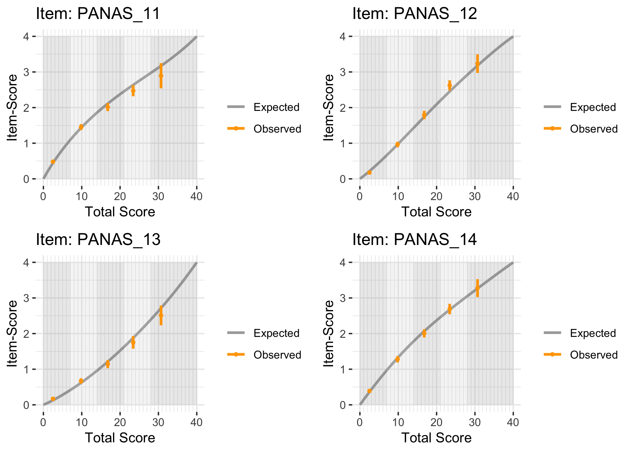
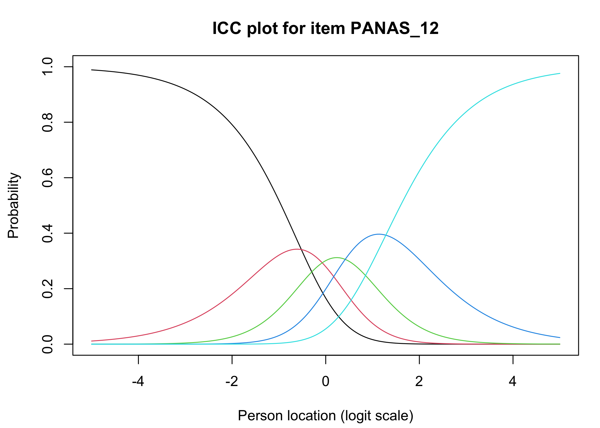
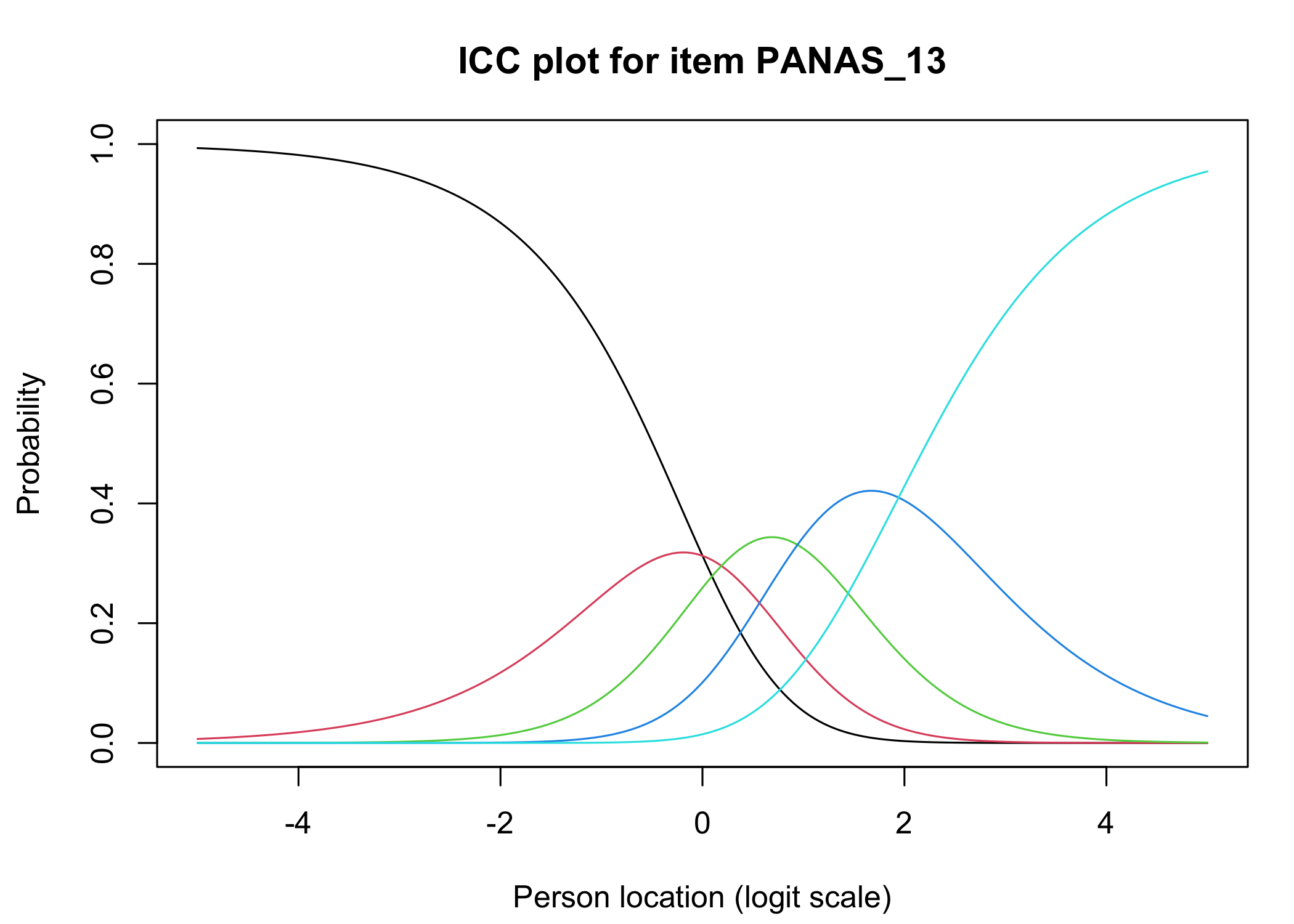
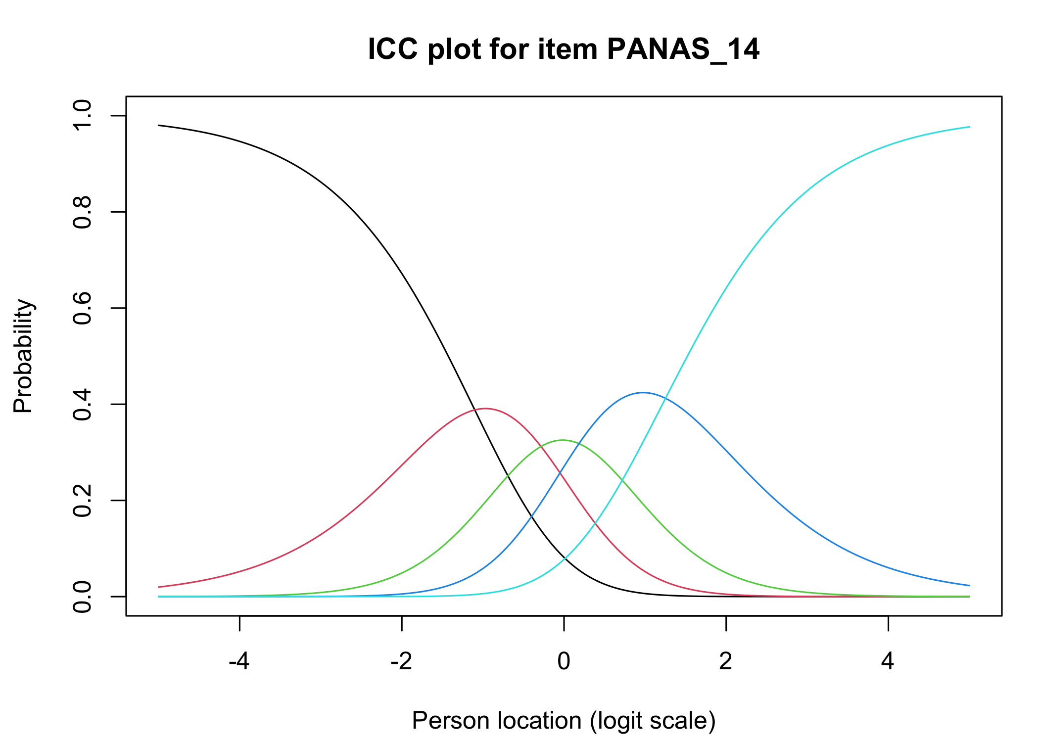
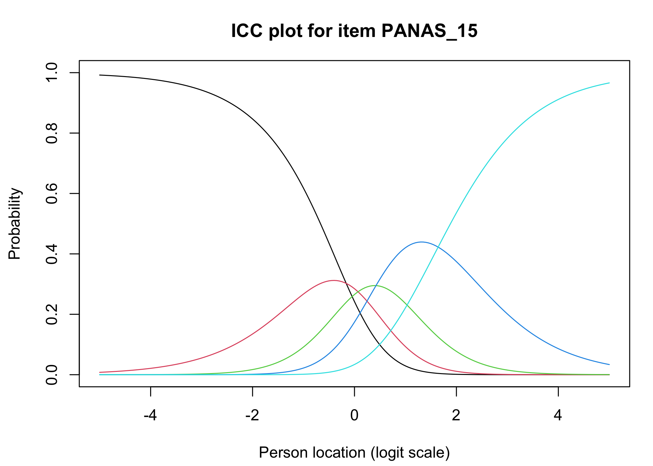
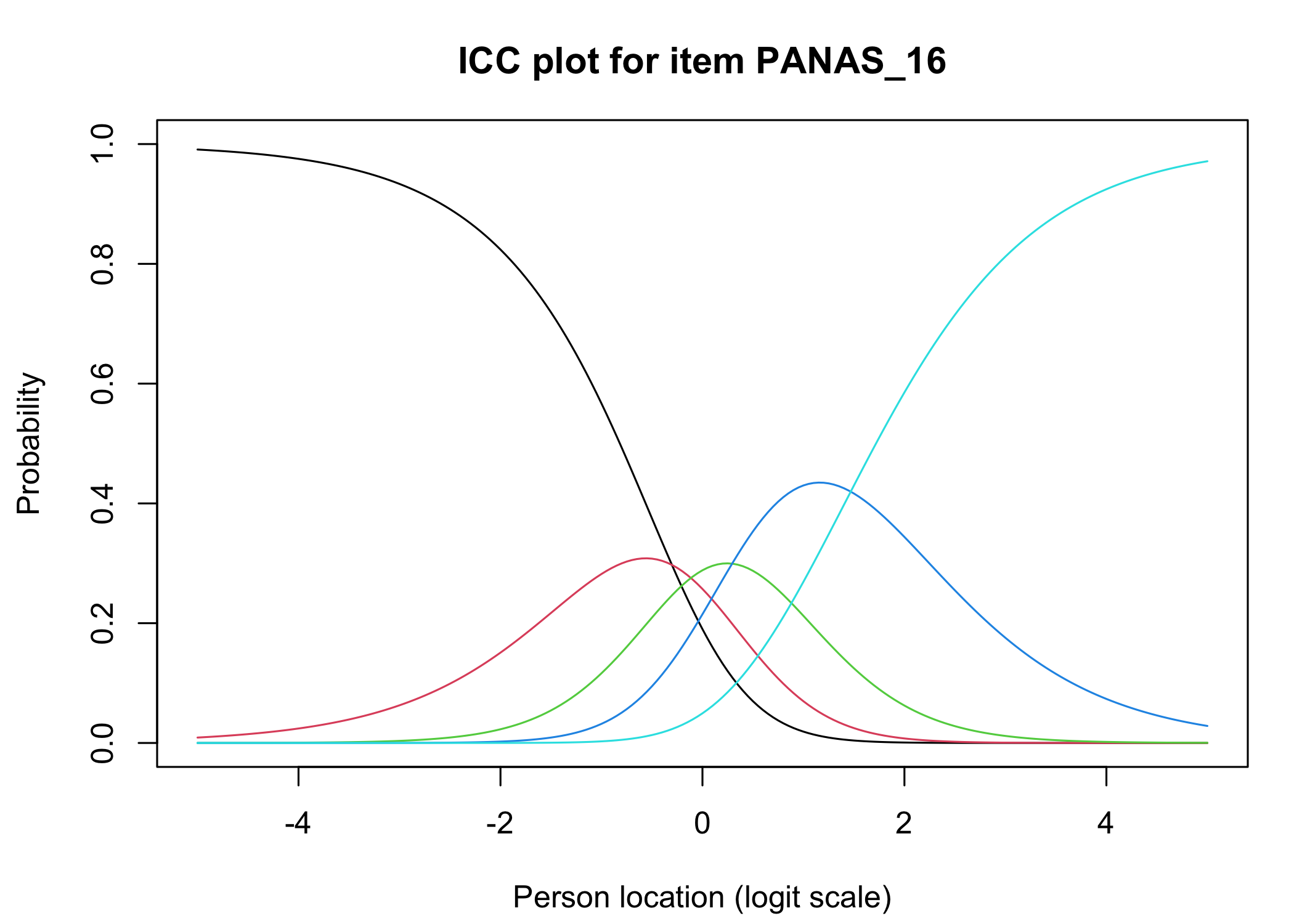
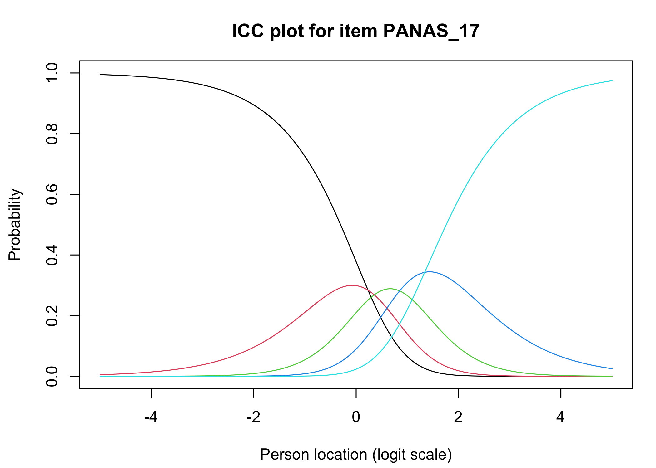
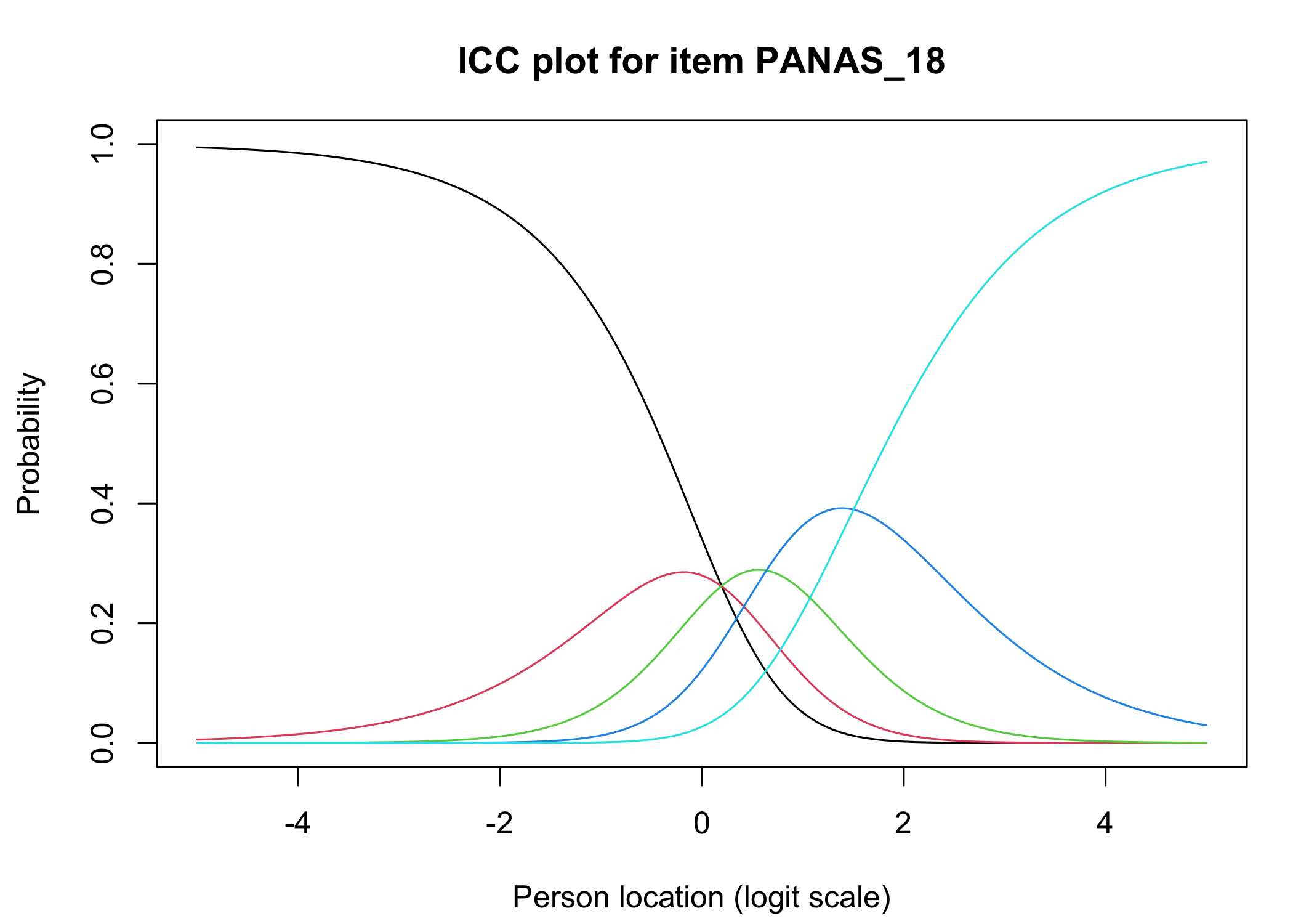
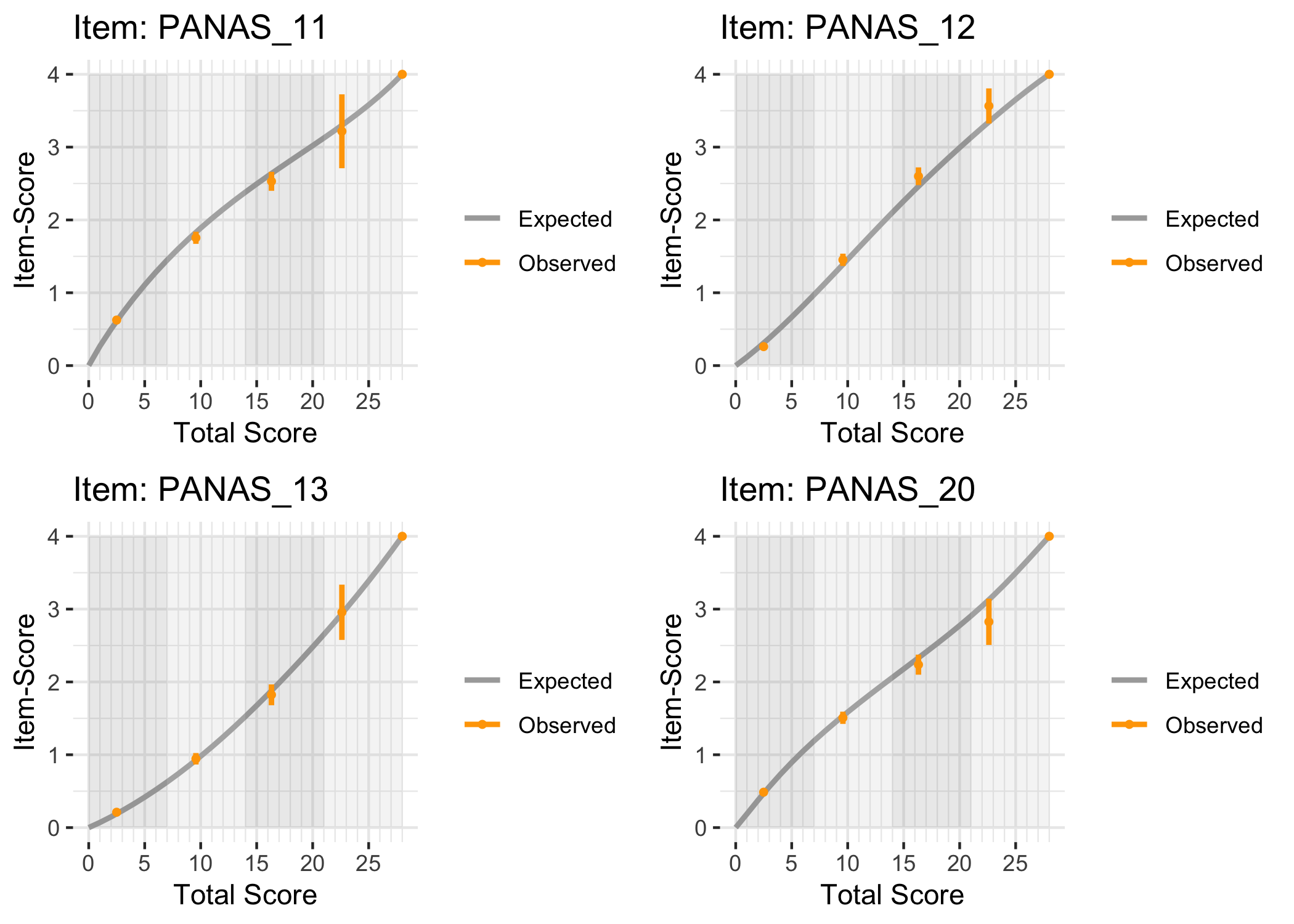
### Conditional item characteristic curves
The [`iarm`](https://cran.r-project.org/web/packages/iarm/index.html) package [@mueller_iarm_2022] provides several interesting functions for assessing item fit, DIF and other things. Some of these functions have been implemented in simplified versions in `easyRasch`, and others may be included in a future version. Below are conditional item characteristic curves (ICC's) using the estimated theta (factor score).
These curves indicate item fit on a group level, where respondents are split into "class intervals" based on their sum score/factor score.
```{r}
RIciccPlot(df) +
  guide_area() # this relocates the legend/guide, which may produce a nicer output
```
A similar visualization, even more informative and flexible, has been made available in the [`RASCHplot`](https://github.com/ERRTG/RASCHplot/) package [@buchardt_visualizing_2023]. The package needs to be installed from GitHub (see commented code below). The linked paper is recommended reading, not least for descriptions of the useful options available. Below are some sample plots showing conditional ICC's using the raw sum score.
```{r}
library(RASCHplot) # devtools::install_github("ERRTG/RASCHplot")

CICCplot(PCM(df),
         which.item = c(1:4),
         lower.groups = c(0,7,14,21,28),
         grid.items = TRUE)
```
### PCA of residuals
Principal Component Analysis of Rasch model residuals (PCAR).
```{r}
RIpcmPCA(df)
```
Based on an old rule-of-thumb, the first eigenvalue should be below 1.5 to support unidimensionality [@smith_detecting_2002]. However, as with many other metrics the expected PCAR eigenvalue is also dependent on sample size and test length [@chou_checking_2010]. To be clear, there is no single or easily calculated rule-of-thumb critical value for the largest PCA eigenvalue that will be generally applicable. A parametric bootstrap function has been implemented in `easyRasch` to determine a potentially appropriate cutoff value for the largest PCAR eigenvalue, but it has not been systematically evaluated yet. Below is an example, illustrated with a histogram of the simulated distribution of largest eigenvalues, the 99th percentile and the max value.
```{r}
pcasim <- RIbootPCA(df, iterations = 500, cpu = 8)
hist(pcasim$results, breaks = 50)
pcasim$p99
pcasim$max
```
If the bootstrap turns out to provide an appropriate cutoff value, it still needs to be used together with checking item fit (or item-restscore) and residual correlations (local dependence) to evaluate unidimensionality.
The PCA eigenvalues are mostly included here for those coming from Winsteps who may be looking for this metric. Speaking of Winsteps, the "explained variance" generated by `RIpcmPCA()` will not be comparable to Winsteps corresponding metric, since this function only shows the results from the analysis of residuals and not the variance explained by the Rasch model itself. Additionally, it should be noted that the PCA rotation is set to "oblimin".
### Conditional LRT
The Conditional Likelihood Ratio Test [CLRT, @andersen_goodness_1973] is a global test of fit and can be a useful addition to more informative item-level metrics [@johansson_detecting_2025]. CLRT compares the responses of those scoring below the median to those scoring above the median to assess the homogeneity of the test. Below, we run the test using the smaller sample with a function from the `iarm` package.
```{r}
clr_tests(df500, model = "PCM")
```
The test is clearly statistically significant, even with the smaller sample, which indicates that unidimensionality does not hold. However, CLRT is sensitive to large sample sizes and number of items, and produces false positives above the nominal 5% level. See <https://pgmj.github.io/clrt.html> for a very small simulation study. To minimize the sample size issue, a non-parametric bootstrap function has been implemented in `easyRasch`, where one can set the sample size manually. The function will then sample with replacement from the response data and conduct a separate CLRT for each sample drawn.
```{r}
RIbootLRT(df, iterations = 1000, samplesize = 400, cpu = 8)
```
The bootstrap method also shows a strong majority of statistically significant results.
Global tests do not provide any information about the reason for misfit. The `iarm` package has also implemented a function to get item specific information related to the CLRT, showing observed and expected values for each item.
```{r}
item_obsexp(PCM(df500))
```
### Local dependence (Q~3~)
In order to support unidimensionality, items should only be related to each other through the latent variable, and otherwise be independent of each other. This is called "local independence" when fulfilled and "local dependence" (LD) when there are issues. The extreme case of dependence is when all respondents give the same response for two items. Two aspects of LD are often described [@chen_local_1997]:
1. Underlying local dependence (ULD), which is when the locally dependent items are measuring a different latent variable than the other items.
2. Surface local dependence (SLD), when item content is very similar.
By investigating patterns in model residuals, we can determine whether items are independent or not. There are several tests that can be used to assess LD, of which Yen's Q~3~ generally has good properties. Please see [@edwards_diagnostic_2018] for an overview of different methods. It is recommended to use multiple methods, since they may perform differently with different types of LD. For instance, Chen & Thissen [-@chen_local_1997] report that G^2^ is slightly more powerful than Yen's Q~3~ in detecting SLD, while the reverse is true for ULD.
Similarly to item fit, we need to run simulations based on the observed data to get a useful cutoff threshold value for when residual correlations amongst item pairs are larger than would be expected from items that fit a unidimensional Rasch model [@christensen2017].
The simulation/bootstrap procedure can take some time to run, depending on the complexity of your data, but it is necessary to set the appropriate cutoff value. The number of iterations to use has yet to be systematically evaluated, but I recommend no less than 500, and at least 1000 as a starting point.
```{r}
simcor1 <- RIgetResidCor(df, iterations = 500, cpu = 8)
RIresidcorr(df, cutoff = simcor1$p995)
```
The matrix above shows item-pair correlations of item residuals, with highlights in red showing correlations crossing the threshold compared to the average item-pair correlation (for all item-pairs) [@christensen2017]. The threshold used in the example above has selected the 99.5th percentile from the simulations. The `simcor1` object also pre-calculates values for the 95th, 99th, 99.5th and 99.9th percentiles as well as the maximum. If you desire another percentile, you can manually calculate it from the results in the `simcor1` object using `quantile()`.
Rasch model residual correlations using Yen's Q~3~ are calculated using the [mirt](https://cran.r-project.org/web/packages/mirt/index.html) package.
### Local dependence (G^2^)
Rasch model residual correlations using Chen & Thissen's G^2^ are calculated using the [mirt](https://cran.r-project.org/web/packages/mirt/index.html) package.
```{r}
simcor_g2 <- RIgetResidCorG2(df, iterations = 500, cpu = 8)
RIresidcorrG2(df, cutoff = simcor_g2$p995)
```
### LD (partial gamma)
Another way to assess local (in)dependence is by partial gamma coefficients [@kreiner_analysis_2004]. This is also a function from the `iarm` package. See `?iarm::partgam_LD` for details.
```{r}
RIpartgamLD(df)
```
### 1st contrast loadings
```{r}
RIloadLoc(df)
```
Here we see item locations and their loadings on the first residual contrast. This figure can be helpful to identify clusters in data or multidimensionality. You can get a table with standardized factor loadings using `RIloadLoc(df, output = "table")`.
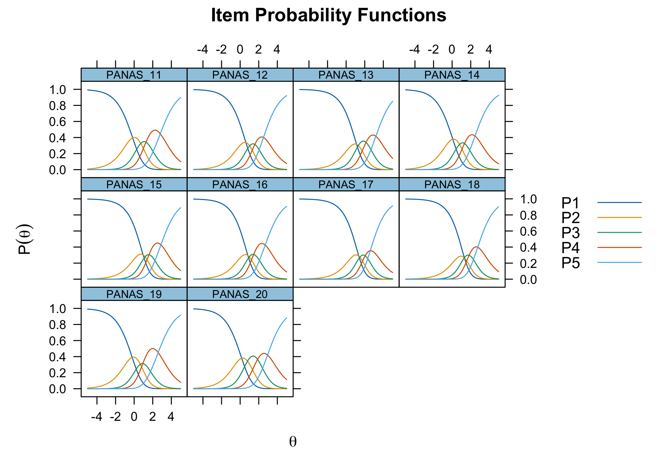
### Analysis of response categories
The `xlims` setting changes the x-axis limits for the plots. The default values usually make sense, and we mostly add this option to point out the possibility of doing so. You can also choose to only show plots for only specific items.
```{r}
#| layout-ncol: 2
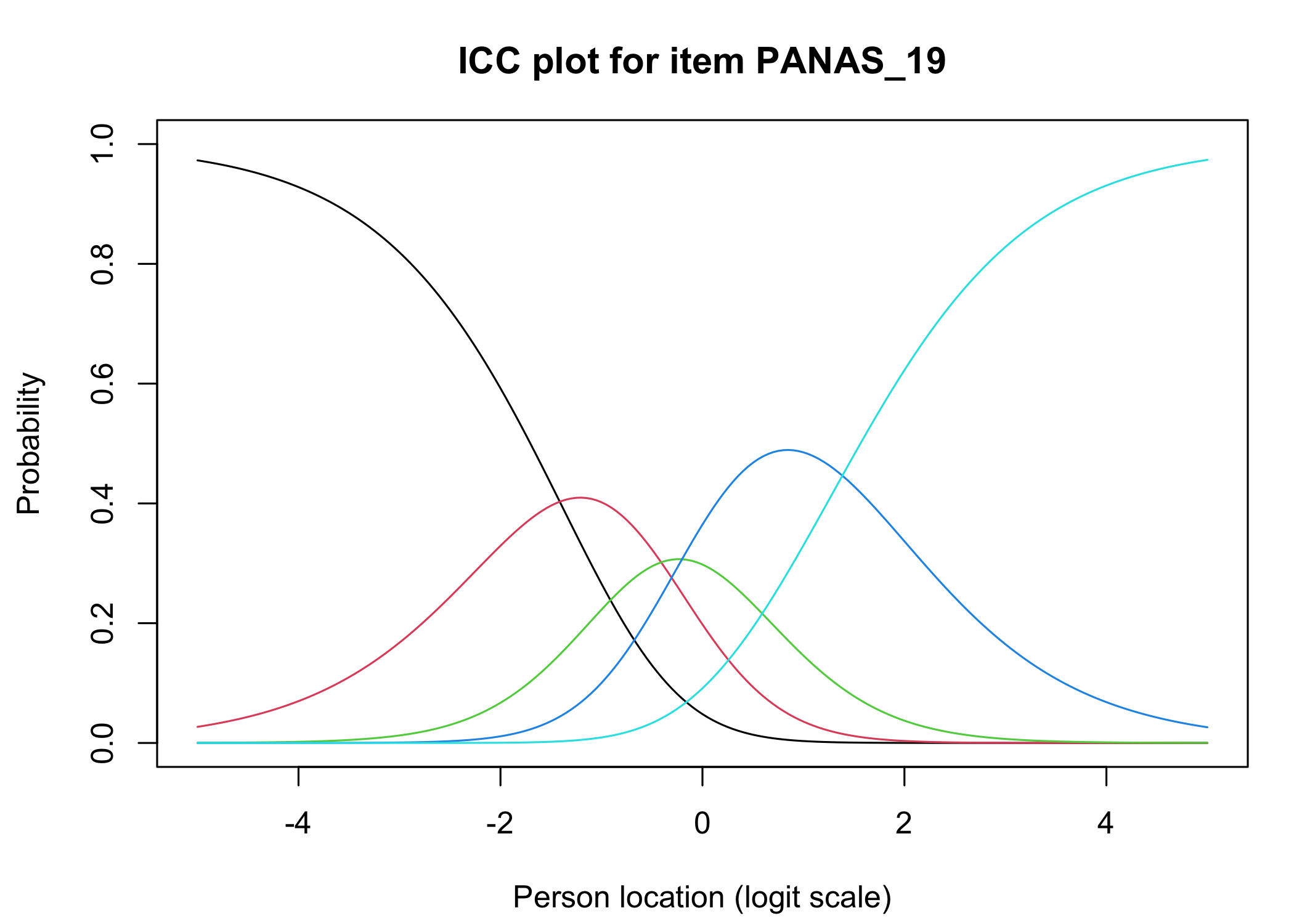
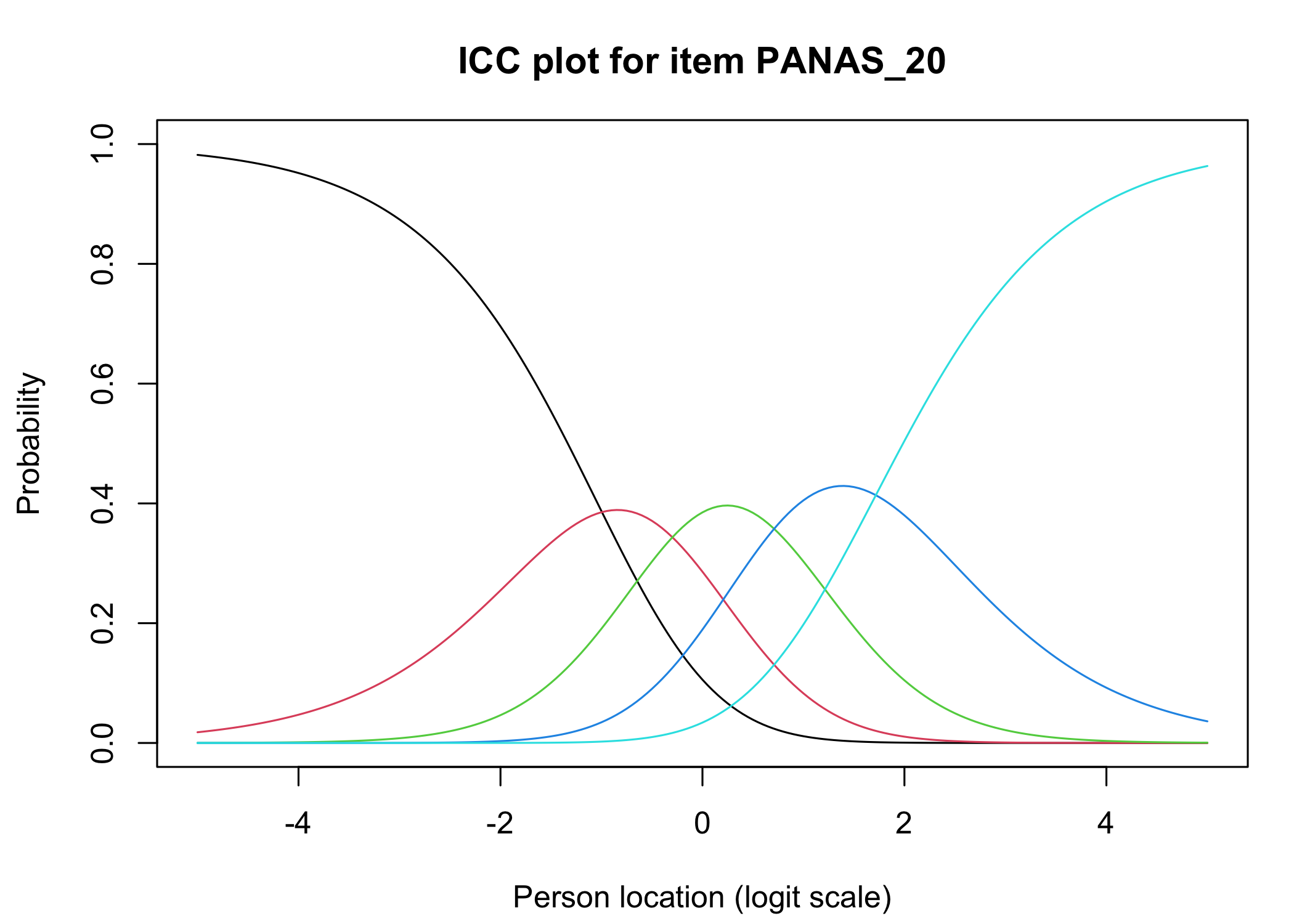
RIitemCats(df, xlims = c(-5,5))
```
Each response category for each item should have a curve that indicates it to be the most probably response at some point on the latent variable (x axis in the figure).
### Response categories MIRT
This produces a single figure with all items. Note that `mirt()` uses marginal maximum likelihood (MML) estimation which may produce slightly different results compared to eRm/CML when the distribution of person locations/scores are non-normal.
```{r}
mirt(df, model=1, itemtype='Rasch', verbose = FALSE) %>%
  plot(type="trace", as.table = TRUE,
       theta_lim = c(-5,5)) # changes x axis limits
```
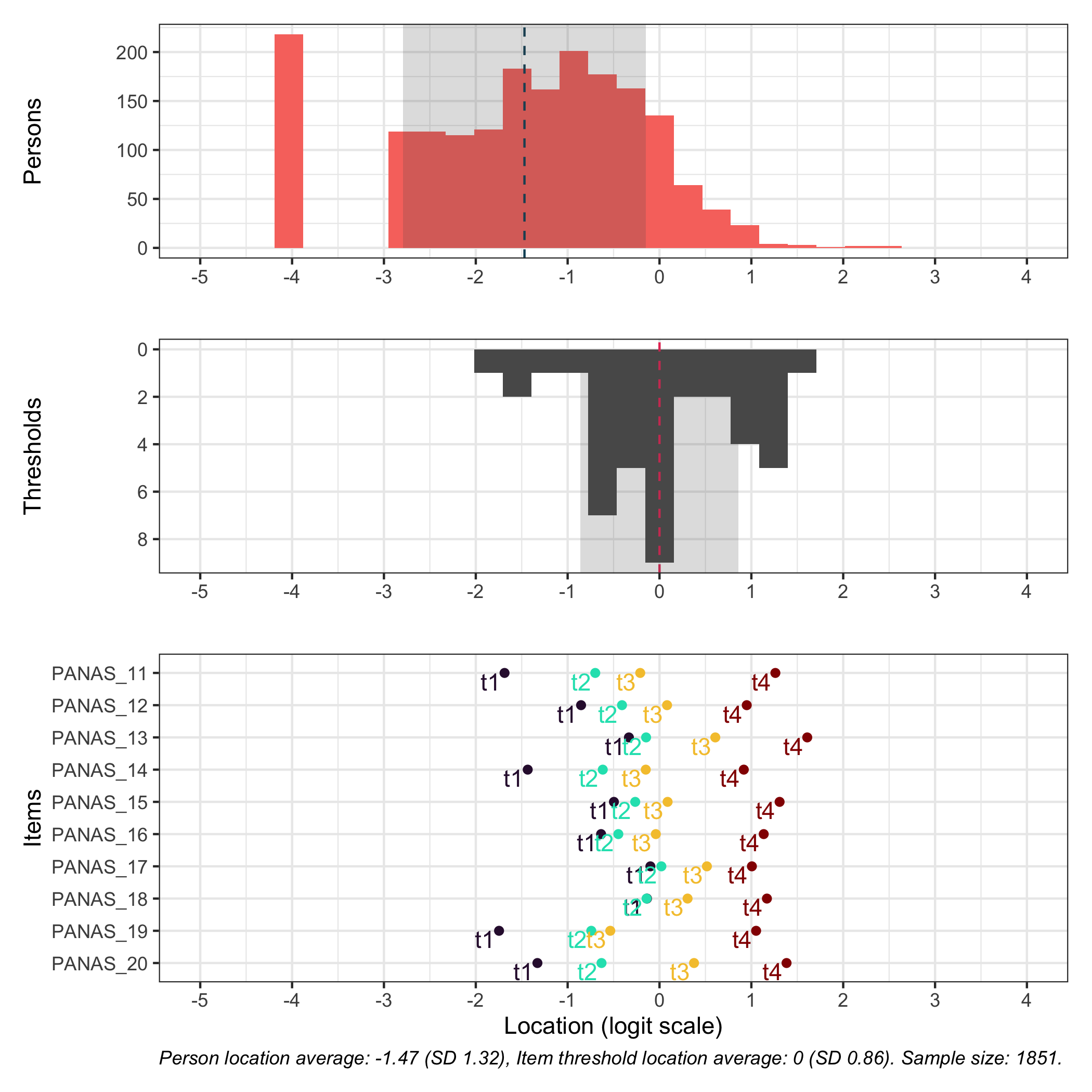
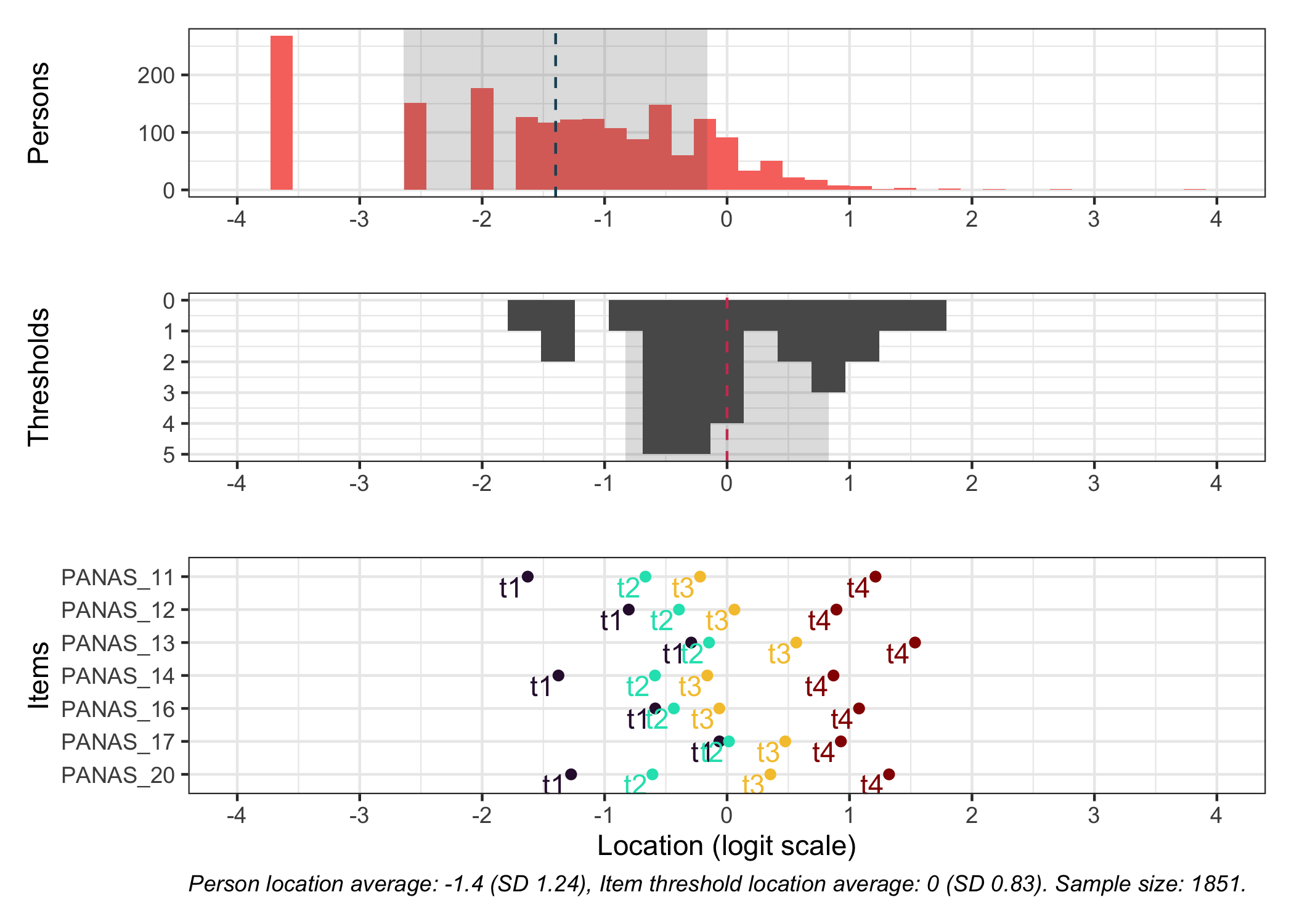
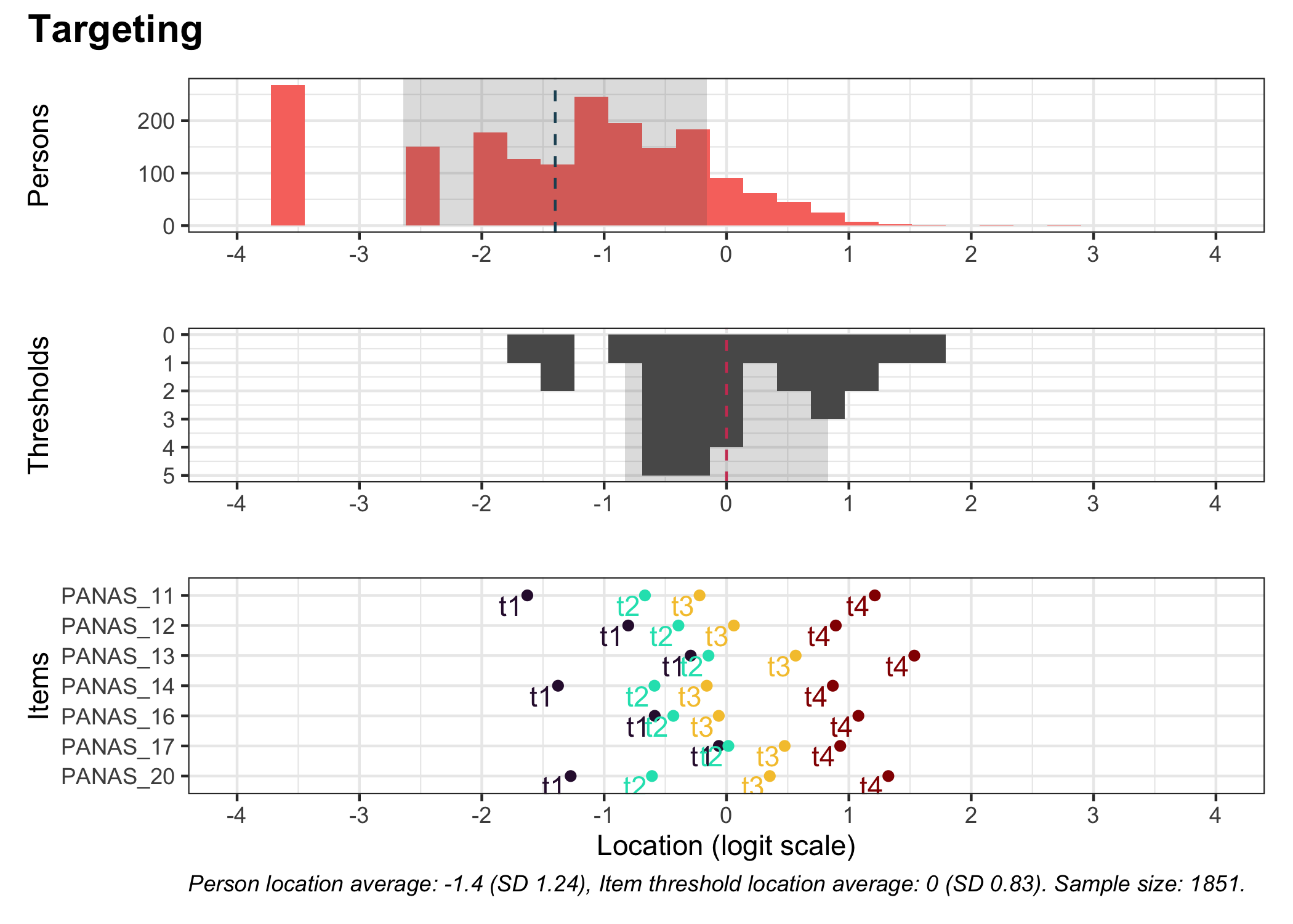
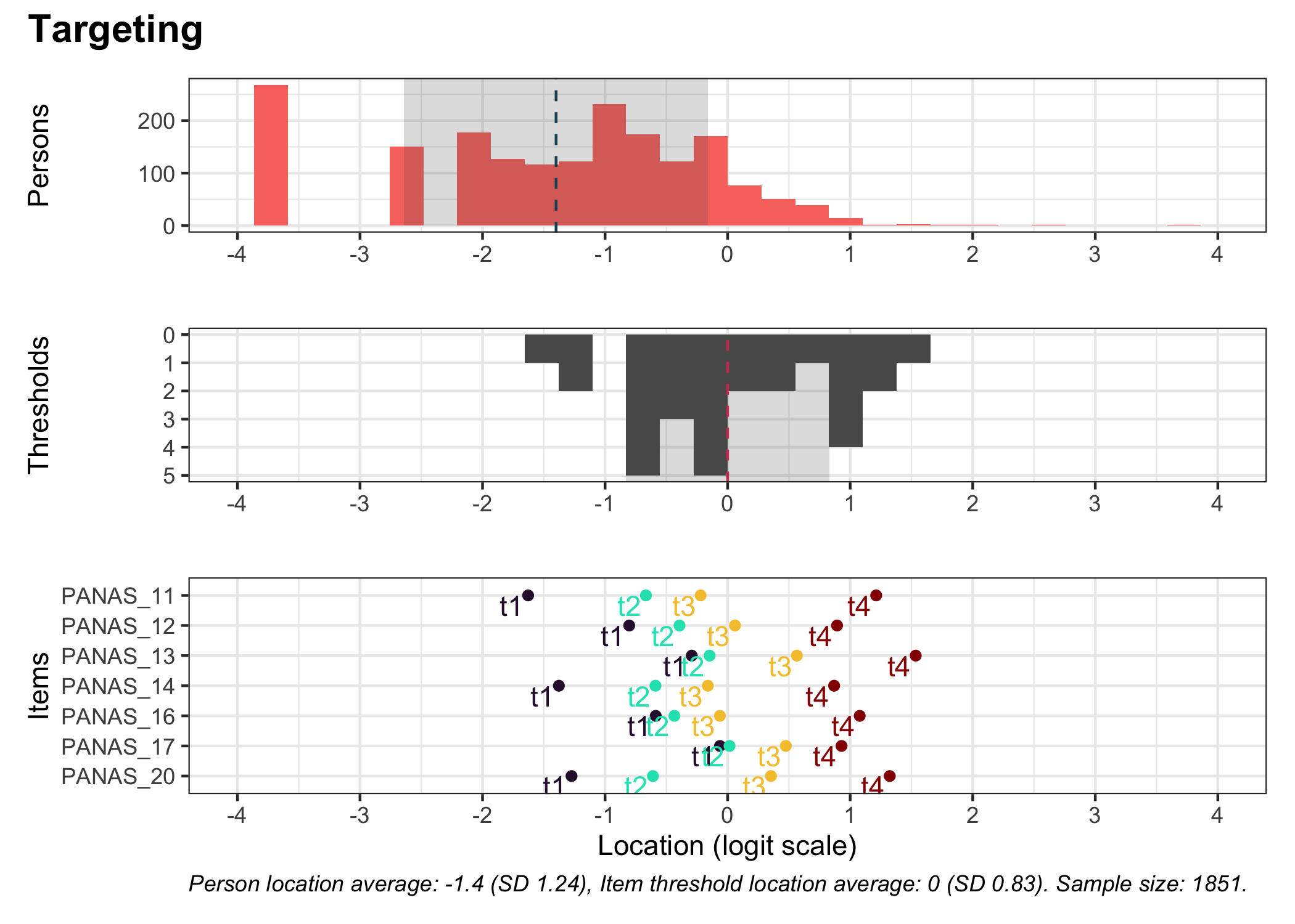
### Targeting
```{r}
#| fig-height: 7
# increase fig-height in the chunk option above if you have many items
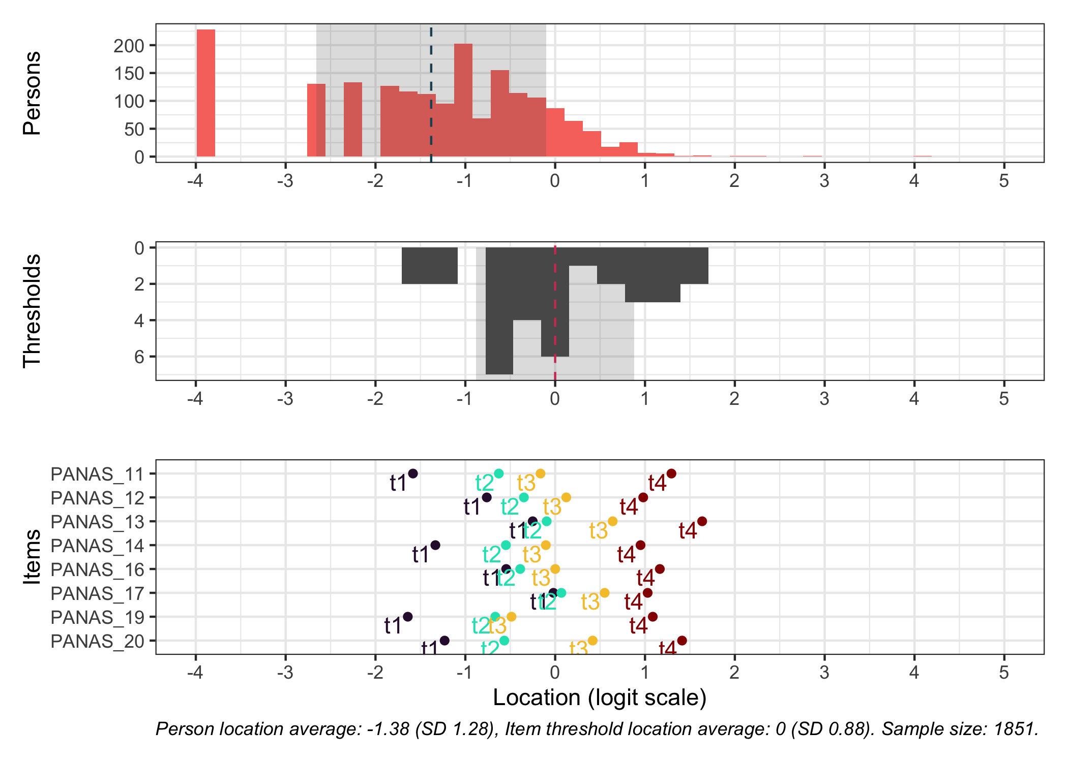
RItargeting(df, xlim = c(-5,4)) # xlim defaults to c(-4,4) if you omit this option
```
This figure shows how well the items fit the respondents/persons. It is a sort of [Wright Map](https://www.rasch.org/rmt/rmt253b.htm) that shows person locations and item threshold locations on the same logit scale.
The top part shows person location histogram, the middle part an inverted histogram of item threshold locations, and the bottom part shows individual item threshold locations. The histograms also show means and standard deviations.
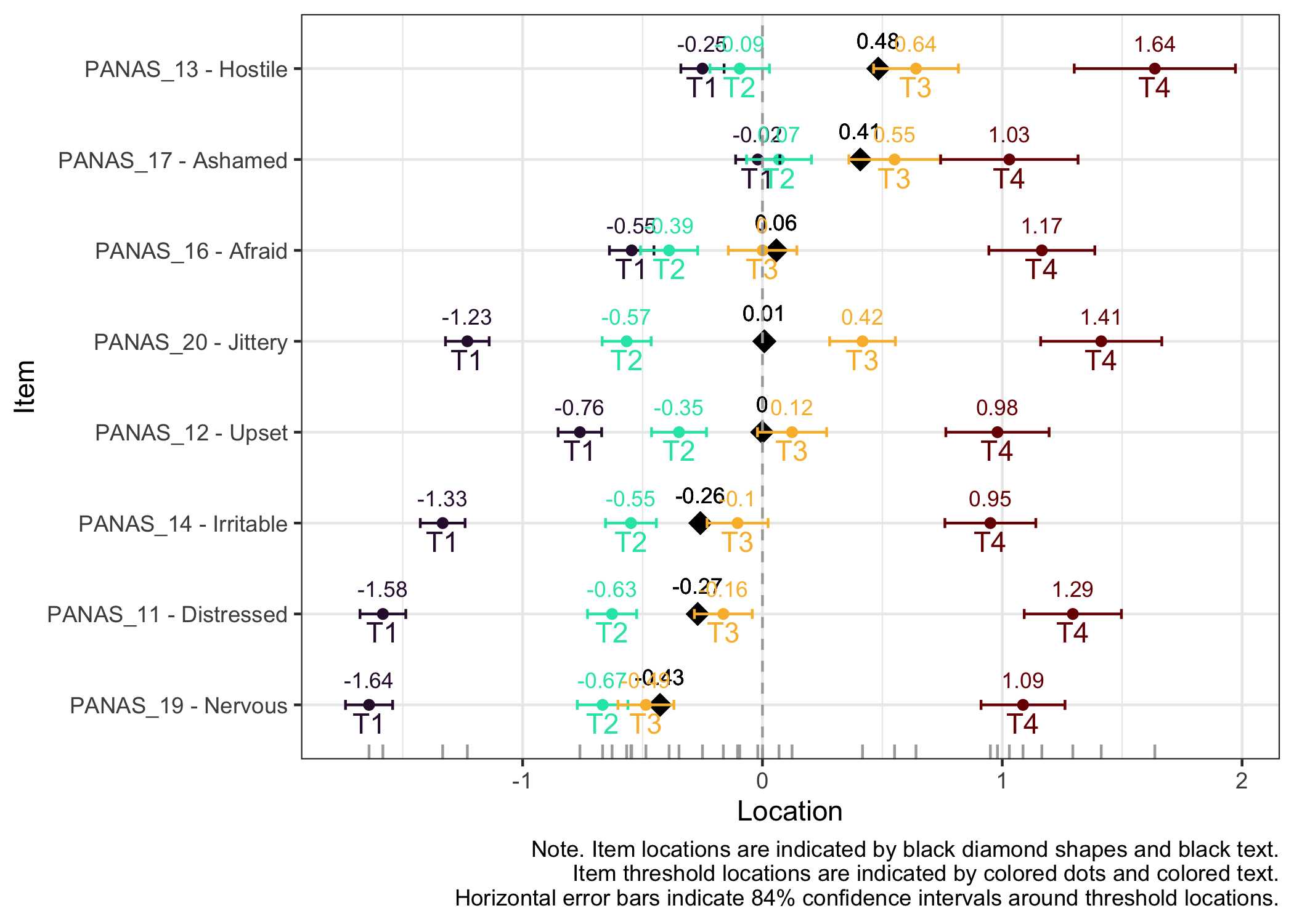
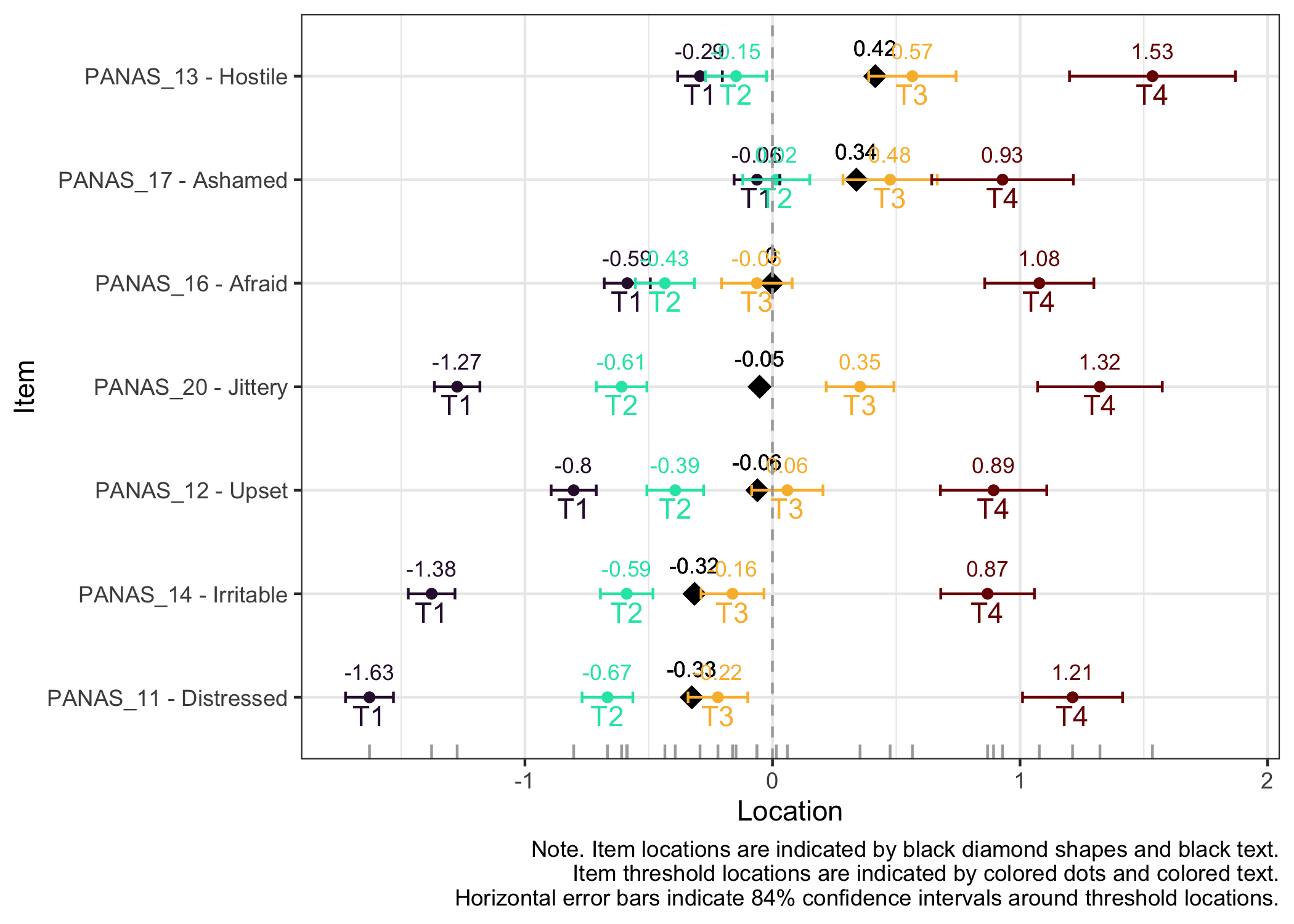
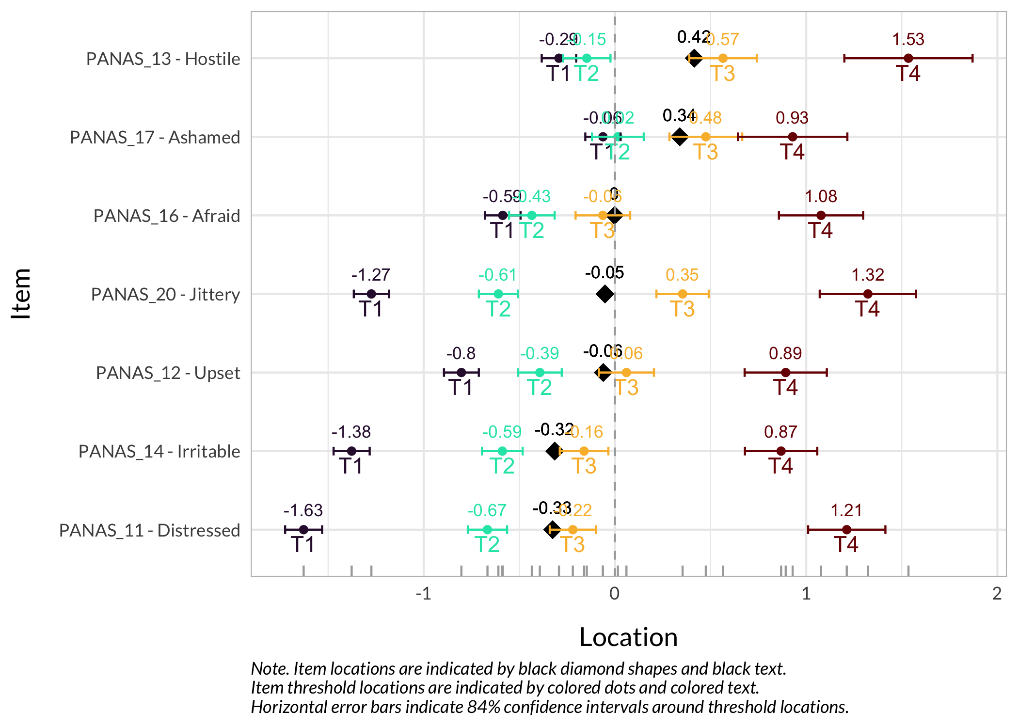
### Item hierarchy
Here the items are sorted on their average threshold location (black diamonds). 84% confidence intervals are shown around each item threshold location. For further details, see the caption text below the figure.
The numbers displayed in the plot can be disabled using the option `numbers = FALSE`.
```{r}
#| fig-height: 6
RIitemHierarchy(df)
```
:::
### Analysis 1 comments
Item fit shows a lot of issues.
Item 18 has issues with the second lowest category being disordered. Several other items have very short distances between thresholds 1 and 2, which is also clearly seen in the Item Hierarchy figure above.
Two item-pairs show residual correlations far above the cutoff value:
- 15 and 16 (scared and afraid)
- 17 and 18 (ashamed and guilty)
Since item 15 also has a residual correlation with item 19, we will remove it. In the second pair, item 18 will be removed since it also has problems with disordered response categories.
::: {.callout-note icon="true"}
We have multiple "diagnostics" to review when deciding which item to remove if there are strong residual correlations between two items. Here is a list of commonly used criteria:
- item fit
- item threshold locations compared to sample locations (targeting)
- ordering of response categories
- DIF
- and whether there are residual correlations between one item and multiple other items
:::
```{r}
removed.items <- c("PANAS_15","PANAS_18")

df_backup <- df
df500_backup <- df500

df <- df_backup %>%
  select(!any_of(removed.items))

df500 <- df500_backup %>%
  select(!any_of(removed.items))
```
As seen in the code above, I chose to create a backup copy of the original dataframes, then removing the items. This can be useful if, at a later stage in the analysis, I want to be able to quickly "go back" and reinstate an item or undo any other change I have made.
## Rasch analysis 2
With items 15 and 18 removed.
```{r}
#| column: margin
#| echo: false
RIlistItemsMargin(df, fontsize = 13)
```
::: panel-tabset
### Item-restscore bootstrap
```{r}
RIbootRestscore(df, iterations = 250, samplesize = 800)
```
### Conditional item fit
Still using the smaller sample of n = 500.
```{r}
simfit2 <- RIgetfit(df500, iterations = 400, cpu = 8)
RIitemfit(df500, simcut = simfit2)
```
### PCA of residuals
```{r}
RIpcmPCA(df)
```
### Residual correlations
```{r}
simcor2 <- RIgetResidCor(df, iterations = 400, cpu = 8)
RIresidcorr(df, cutoff = simcor2$p99)
```
### 1st contrast loadings
```{r}
RIloadLoc(df)
```
### Targeting
```{r}
#| fig-height: 5
RItargeting(df, xlim = c(-4,4), bins = 45)
```
### Item hierarchy
```{r}
#| fig-height: 5
RIitemHierarchy(df)
```
:::
### Analysis 2 comments
Items 16 & 19, and 12 & 14 show problematic residual correlations.
Let's look at DIF before taking action upon this information. **While we are keeping DIF as a separate section in this vignette, it is recommended to include DIF-analysis in the `panel-tabset` above (on item fit, residual correlations, etc).**
## DIF - differential item functioning
DIF is a complex topic, which is why it gets a separate section here. Even so, this vignette will just brush the surface. For an historical overview, which also includes recent developments, see Thissen [-@thissen_review_2025].
::: {.callout-note icon="true"}
While we are keeping DIF as a separate section in this vignette, it is recommended to include DIF-analysis in the parallel analysis above (on item fit, targeting, residual correlations, etc) since DIF tests will help you understand or evaluate item functioning together with the other tests.
:::
We'll be looking at whether item (threshold) locations are stable between demographic subgroups. There are usually two key aspects to this analysis. One is whether we can detect DIF for one or more items. The other is the magnitude of DIF and how it affects the use of the overall test, if test scores are biased for any group. I recommend a paper by Chalmers et al. [-@chalmers_it_2016] on the topic of DTF, differential test functioning.
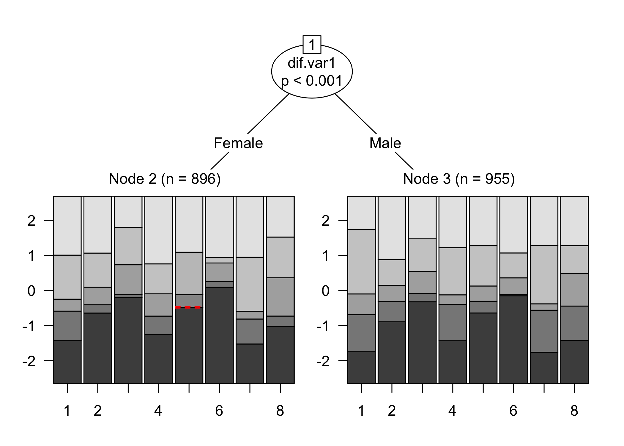
There are several DIF analysis tools available. The first one uses the package `psychotree`, which relies on statistical significance at p < .05 as an indicator for DIF. This is a criterion that is highly sample size sensitive, and we are always interested in the size/magnitude of DIF as well, since that will inform us about the impact of DIF on the estimated latent variable.
The structure of DIF is also important to assess, particularly for polytomous data. Uniform DIF means that the DIF is similar across the latent continuum. The `RIciccPlot()` function can be used for DIF analysis and produces curves that show whether DIF is uniform or not. We can also test for uniformity formally in R using the `lordif` package, as demonstrated in @sec-lordif. However, it should be noted that the `lordif` package does not provide an option to use Rasch models, and there may be results that are caused by also allowing the discrimination parameter to vary across items.
A recent preprint [@henninger_partial_2024] does a great job illustrating "differential step functioning" (DSF), which is when item threshold locations in polytomous data show varying levels of DIF. It also describes a forthcoming development of the `psychotree` where one can use DIF effect size and purification functions to evaluate DIF/DSF. When the updated package is available, I will work to implement these new functions into the `easyRasch` package as well.
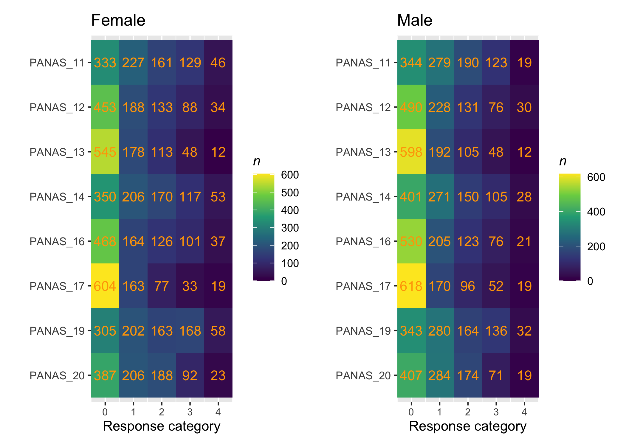
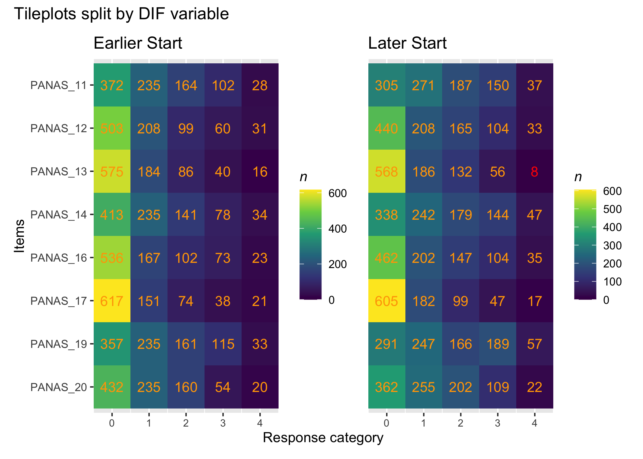
::: {.callout-note icon="true"}
It is important to ensure that no cells in the data are empty for subgroups when conducting a DIF analysis. Split the data using the DIF-variable and create separate tileplots to review the response distribution in the DIF-groups.
:::
```{r}
RIdifTileplot(df, dif$Sex)
```
### Sex
```{r}
#| column: margin
#| echo: false
RIlistItemsMargin(df, fontsize = 13)
```
::: panel-tabset
#### Table
```{r}
#| fig-height: 3
RIdifTable(df, dif$Sex)
```
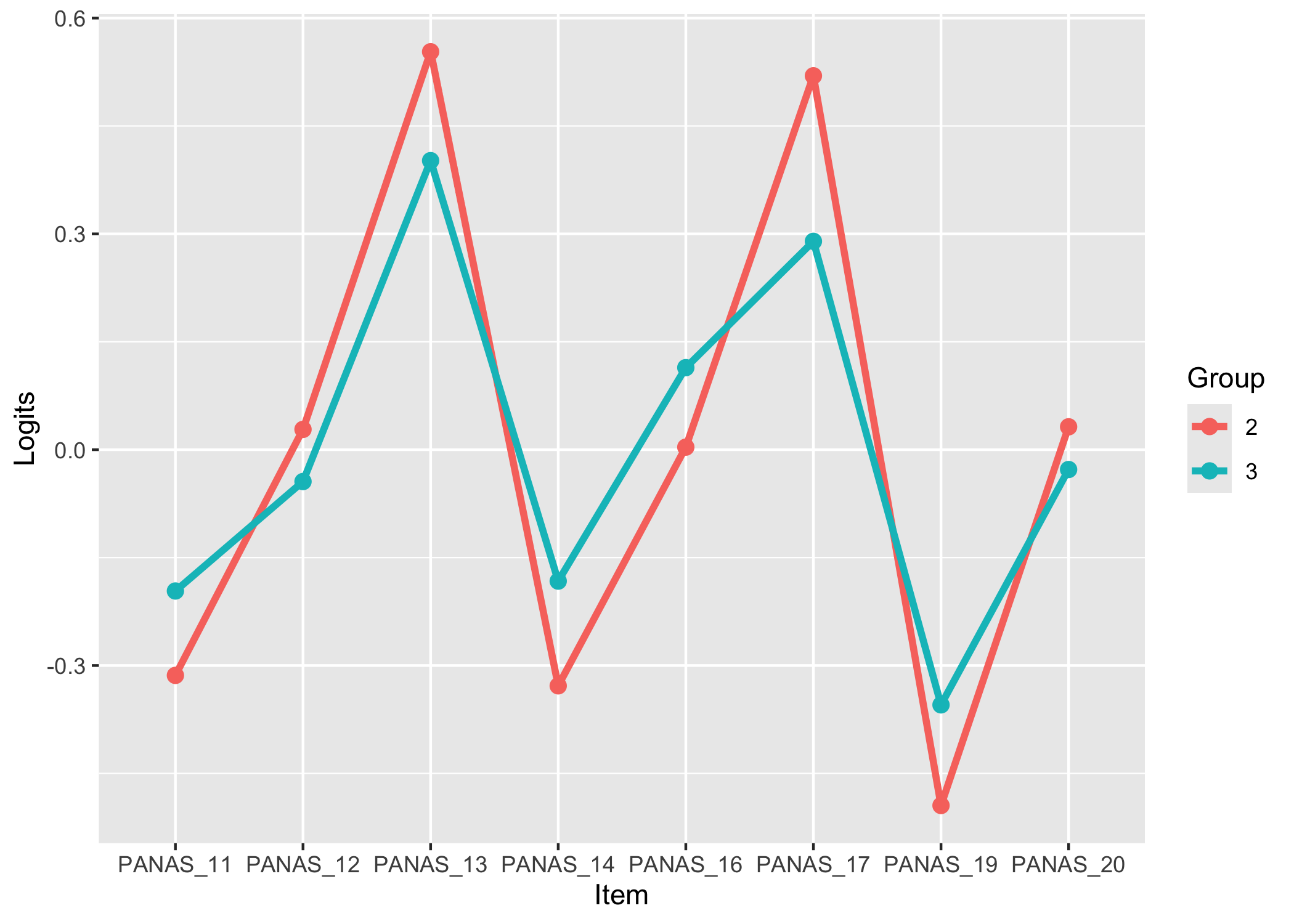
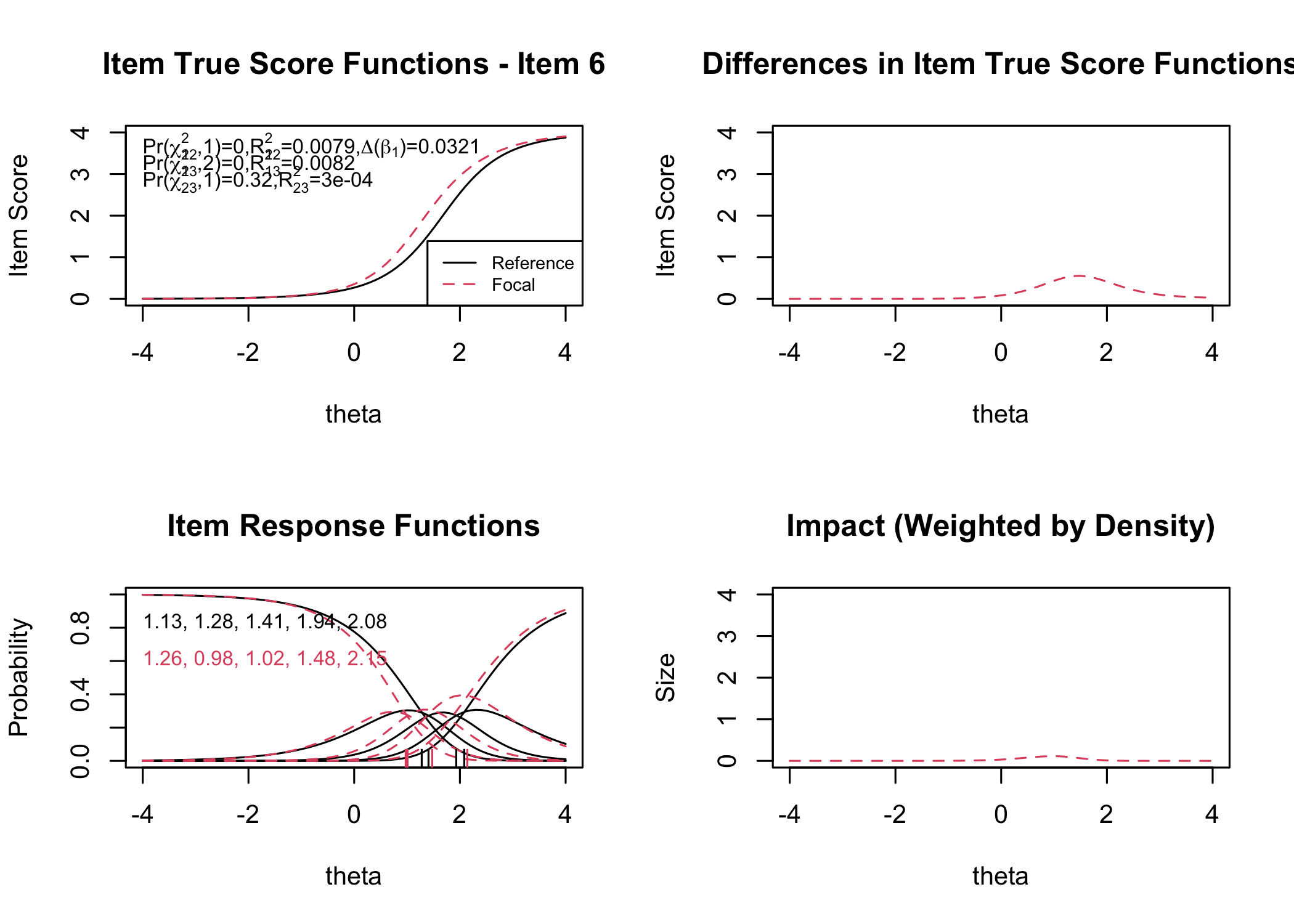
#### Figure items
```{r}
RIdifFigure(df, dif$Sex)
```
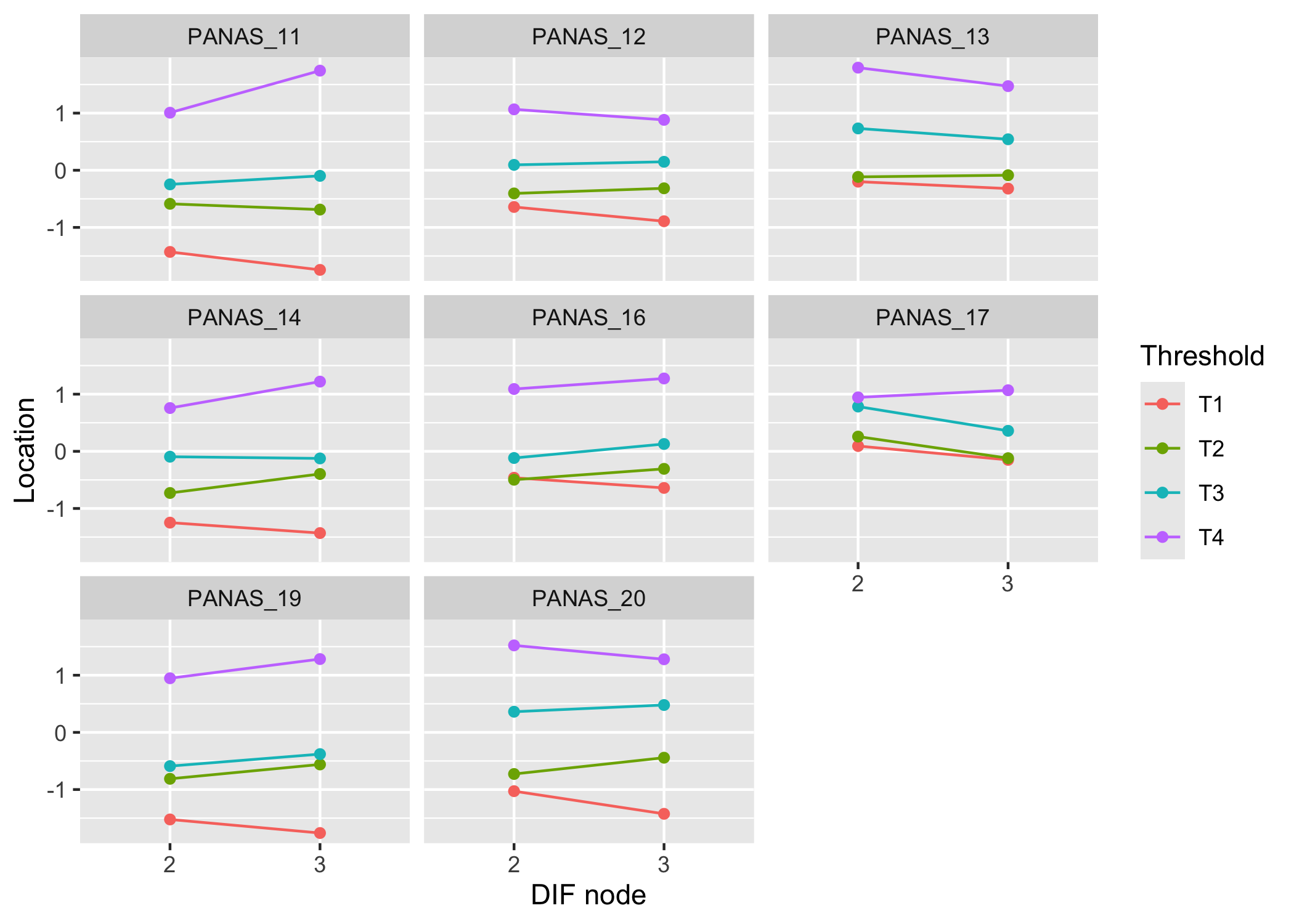
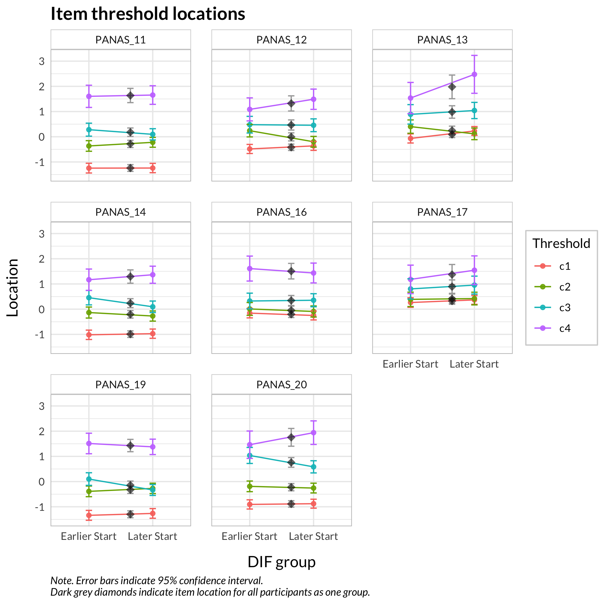
#### Figure thresholds
```{r}
RIdifFigThresh(df, dif$Sex)
```
:::
While no item shows problematic levels of DIF regarding item location, as shown by the table, there is an interesting pattern in the thresholds figure. The lowest threshold seems to be slightly lower for node 3 (Male) for all items. Also, item 11 shows a much wider spread of item locations for node 3 compared to node 2.
The results do not require any action since the difference is small.
### Age
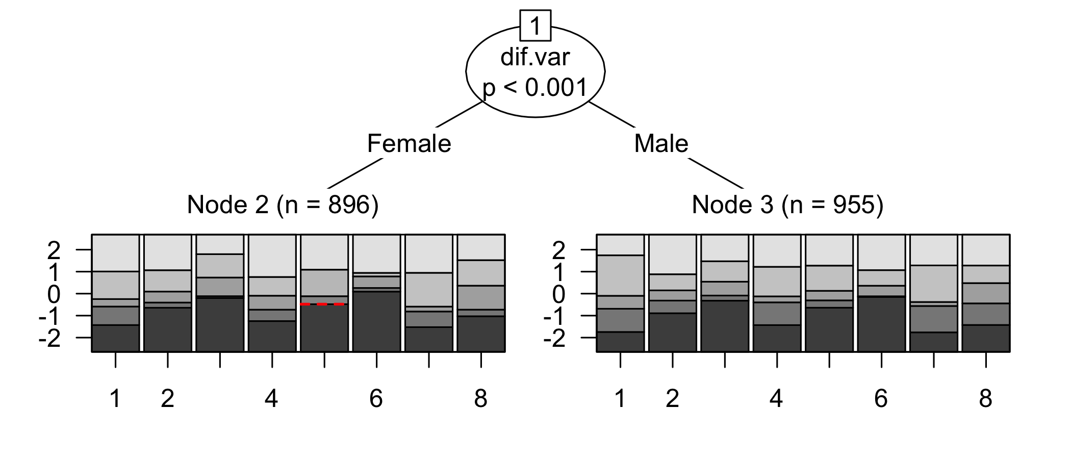
The `psychotree` package uses a model-based recursive partitioning that is particularly useful when you have a continuous variable such as age in years and a large enough sample. It will test different ways to partition the age variable to determine potential group differences [@strobl2015; @strobl2021].
```{r}
RIdifTable(df, dif$Age)
```
No DIF found for age.
### Group
```{r}
RIdifTable(df, dif$Group)
```
And no DIF for group.
### Sex and age
The `psychotree` package also allows for DIF interaction analysis with multiple DIF variables. We can use `RIdifTable2()` to input two DIF variables.
```{r}
RIdifTable2(df, dif$Sex, dif$Age)
```
No interaction effect found for sex and age. The analysis only shows the previously identified DIF for sex.
### LRT-based DIF {#sec-diflrt}
We'll use the group variable as an example. It's always important to review the response distribution across DIF groups prior to running the DIF analysis. We need to make sure that there are responses in all cells in all subgroups.
```{r}
RIdifTileplot(df, dif$Group)
```
First, we can simply run the test to get the overall result.
```{r}
erm.out <- PCM(df)
LRtest(erm.out, splitcr = dif$Group)
```
Review the documentation for further details, using `?LRtest` in your R console panel in Rstudio. There is also a plotting function, `plotGOF()` that may be of interest.
```{r}
#| column: margin
#| echo: false
RIlistItemsMargin(df, fontsize = 13)
```
::: panel-tabset
#### Item location table
```{r}
RIdifTableLR(df, dif$Group)
```
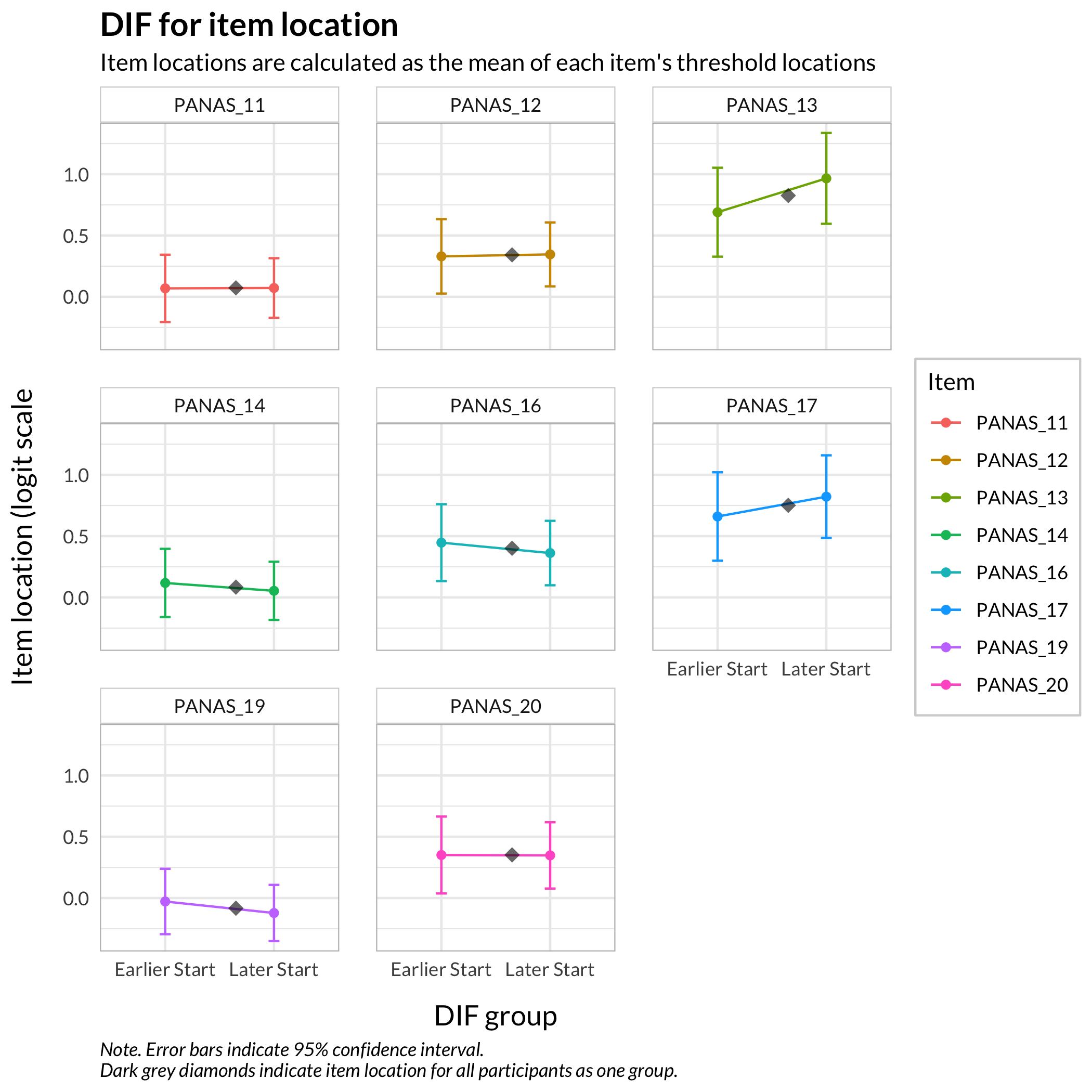
#### Item location figure
```{r}
#| fig-height: 7
RIdifFigureLR(df, dif$Group) + theme_rise()
```
#### Item threshold table
```{r}
RIdifThreshTblLR(df, dif$Group)
```
#### Item threshold figure
```{r}
#| fig-height: 7
RIdifThreshFigLR(df, dif$Group) + theme_rise()
```
:::
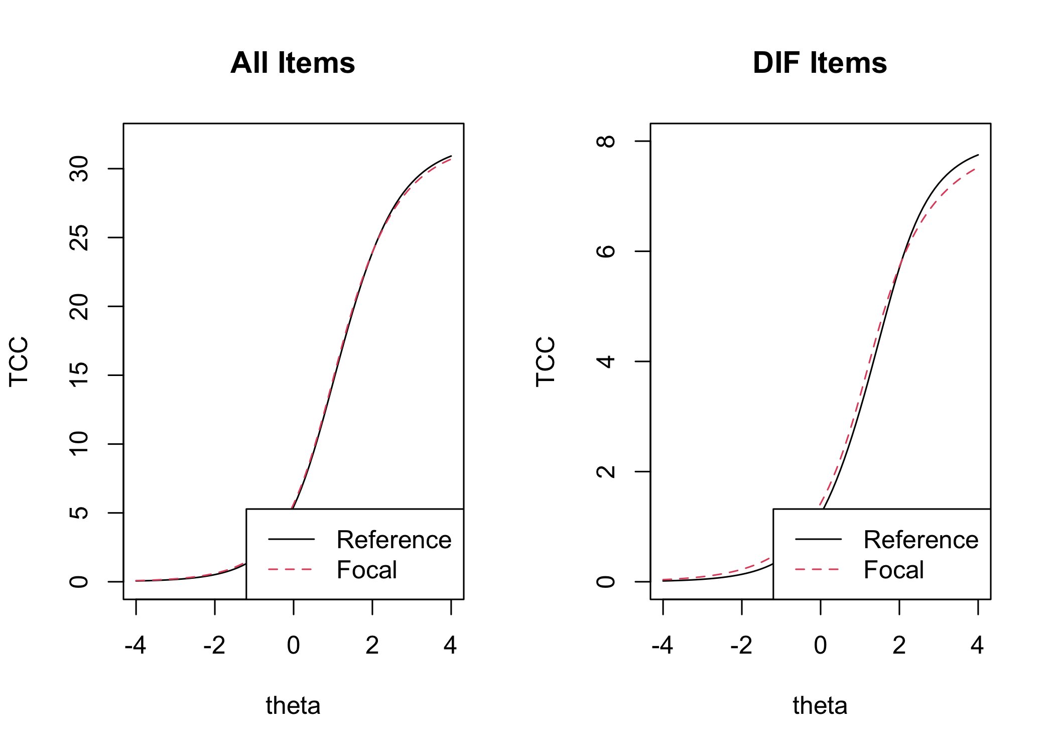
The item threshold table shows that the top threshold for item 13 differs more than 0.5 logits between groups. In this set of 8 items with 4 thresholds each, it is unlikely to result in problematic differences in estimated person scores.
### Conditional ICC
The `iarm` package function for CICC plots also includes the option to use a DIF variable. This gives us information about DIF across the latent continuum when class intervals are created based on latent score groups. If your analysis contains two groups and the lines for the groups cross each other, DIF is non-uniform.
```{r}
RIciccPlot(df, dif = "yes", dif_var = dif$Sex)
```
### Logistic Ordinal Regression DIF {#sec-lordif}
The `lordif` package [@choi_lordif_2011] does not use a Rasch measurement model, it only offers a choice between the Graded Response Model (GRM) and the Generalized Partial Credit Model (GPCM). Both of these are 2PL models, meaning that they estimate a discrimination parameter for each item in addition to the item threshold parameters. `lordif` relies on the `mirt` package.
There are several nice features available in the `lordif` package. First, we get a χ2 test of uniform or non-uniform DIF. Second, there are three possible methods/criteria for flagging items with potential DIF. One of these uses a likelihood ratio (LR) χ2 test, while the other two are indicators of DIF size/magnitude, either using a pseudo R2 statistic ("McFadden", "Nagelkerke", or "CoxSnell") or a Beta criterion. For further details, see `?lordif` in your R console or the paper describing the package [@choi_lordif_2011].
Below is some sample code to get you started with `lordif`.
```{r}
#| results: hide
library(lordif)

g_dif <- lordif(as.data.frame(df), as.numeric(dif$Sex), # make sure that the data is in a dataframe-object and that the DIF variable is numeric
                criterion = c("Chisqr"),
                alpha = 0.01,
                beta.change = 0.1,
                model = "GPCM",
                R2.change = 0.02)

g_dif_sum <- summary(g_dif)
```
```{r}
# threshold values for colorizing the table below
alpha = 0.01
beta.change = 0.1
R2.change = 0.02

g_dif_sum$stats %>%
  as.data.frame() %>%
  select(!all_of(c("item","df12","df13","df23"))) %>%
  round(3) %>%
  add_column(itemnr = names(df), .before = "ncat") %>%
  mutate(across(c(chi12,chi13,chi23), ~ cell_spec(.x,
                               color = case_when(
                                 .x < alpha ~ "red",
                                 TRUE ~ "black"
                               )))) %>%
  mutate(across(starts_with("pseudo"), ~ cell_spec(.x,
                               color = case_when(
                                 .x > R2.change ~ "red",
                                 TRUE ~ "black"
                               )))) %>%
  mutate(beta12 =  cell_spec(beta12,
                               color = case_when(
                                 beta12 > beta.change ~ "red",
                                 TRUE ~ "black"
                               ))) %>%
  kbl_rise()
```
We can review the results regarding uniform/non-uniform DIF by looking at the `chi*` columns. Uniform DIF is indicated by column `chi12` and non-uniform DIF by `chi23`, while column `chi13` represents "an overall test of "total DIF effect" [@choi_lordif_2011].
While the table indicates significant chi2-tests for items 11 and 17, the magnitude estimates are low for these items.
There are some plots available as well, using the base R `plot()` function. For some reason the plots won't render in this Quarto document, so I will try to sort that out at some point.
```{r}
#| layout-ncol: 2
plot(g_dif) # use option `graphics.off()` to get the plots rendered one by one
#plot(g_dif, graphics.off())
```
### Partial gamma DIF
The `iarm` package provides a function to assess DIF by partial gamma [@bjorner_differential_1998]. It should be noted that this function only shows a single partial gamma value per item, so if you have more than two groups in your comparison, you will want to also use other methods to understand your results better.
There are some recommended cutoff-values mentioned in the paper above:
No or negligible DIF:
- Gamma within the interval -0.21 to 0.21, *or*
- Gamma not significantly different from 0
Slight to moderate DIF:
- Gamma within the interval -0.31 to 0.31 (and outside -0.21 to 0.21), *or*
- not significantly outside the interval -0.21 to 0.21
Moderate to large DIF:
- Gamma outside the interval -0.31 to 0.31, **and**
- significantly outside the interval -0.21 to 0.21
```{r}
RIpartgamDIF(df, dif$Sex)
```
We can see "slight" DIF for item 17, with a statistically significant gamma of .23.
## Rasch analysis 3
While there were no significant issues with DIF for any item/subgroup combination, we need to address the previously identified problem:
- Items 16 and 19 have the largest residual correlation.
We'll remove item 19 since item 16 has better targeting.
```{r}
removed.items <- c(removed.items,"PANAS_19")

df <- df_backup %>%
  select(!any_of(removed.items))

df500 <- df500_backup %>%
  select(!any_of(removed.items))
```
```{r}
#| column: margin
#| echo: false
RIlistItemsMargin(df, fontsize = 13)
```
::: panel-tabset
### Item-restscore bootstrap
```{r}
RIbootRestscore(df, iterations = 250, samplesize = 800)
```
### Item fit
```{r}
simfit3 <- RIgetfit(df500, iterations = 200, cpu = 8)
RIitemfit(df500, simfit3)
```
### CICC
```{r}
RIciccPlot(df)
```
### Residual correlations
```{r}
simcor3 <- RIgetResidCor(df, iterations = 400, cpu = 8)
RIresidcorr(df, cutoff = simcor3$p99)
```
### LRT
```{r}
RIbootLRT(df, iterations = 1000, samplesize = 400, cpu = 8)
```
### Targeting
```{r}
#| fig-height: 5
RItargeting(df, bins = 45)
```
### Item hierarchy
```{r}
#| fig-height: 5
RIitemHierarchy(df)
```
:::
### Analysis 3 comments
There are still problematic residual correlations and some items show misfit (most notably item 12 being overfit), but we will end this sample analysis here and move on to show other functions.
There are several item thresholds that are very closely located, as shown in the item hierarchy figure. This is not ideal, since it will inflate reliability estimates. However, we will not modify the response categories for this analysis, we only note that this is not workable and should be dealt with by trying variations of merged response categories to achieve better separation of threshold locations without disordering.
## Reliability
Reliability (or measurement uncertainty) is often reported as a point estimate only, which implies constant reliability across the latent variable. This does not reflect the targeting aspect and the limitations of reliability often found at the lower and upper regions of the latent continuum. One way to try to better describe the varying reliability is by using the Test Information Function (TIF), which is a curve. I have previously advocated for reporting the TIF curve, but have also found some unexpected results when using it. When I finally sat down to figure out the issues with TIF, I found a paper showing that it behaves quite erratically, especially with fewer than six or so items [@milanzi_reliability_2015]. While the `RItif()` function remains, I recommend careful use of it, or perhaps not using it at all.
The most commonly used reliability metric in Rasch analysis is the PSI, person separation index. It is however important to note that the PSI excludes extreme values (min/max scores), which explains why it is sometimes quite different from other metrics. The reason for excluding participants is that extreme scores cannot be estimated, they need to be imputed/interpolated along with their corresponding measurement error, which is what is used in the PSI metric.
### RMU --- Relative Measurement Uncertainty
```{r}
rel <- RIreliability(df, draws = 1000)
rel$PSI
rel$RMU
```
The new (since `easyRasch` 0.4.0) function `RIreliability()` will produce several estimates of reliability. The potentially most useful metric is a new one, based on a recent preprint [@bignardi_general_2025] which describes a general reliability metric that includes uncertainty around the point estimate, called *RMU, "Relative Measurement Uncertainty"*. Bignardi and colleagues use Bayesian estimation and posterior draws of each respondents latent scores (thetas/locations) to determine the mean and 95% highest density continuous interval (HDCI) of the distribution of correlations between draws [@bignardi_general_2025]. I have borrowed code that the authors made available, and adapted it to simplify the use by grace of the `mirt` package and its function to generate plausible values [PVs, @mislevy_randomization-based_1991;@wu_role_2005] instead of having to learn to specify Bayesian models. Preliminary investigations indicate similar results for PVs and fully Bayesian model posteriors, see the example code in the documentation `?RIreliability` for an example, and [this blog post](https://pgmj.github.io/reliability.html) for a more extensive investigation. The 95% HDCI is a useful addition, and by using PVs, respondents with extreme values are included in a reasonable way. `RIreliability()` has the setting `estim` to choose method of estimation for thetas/latent scores used for the RMU, which uses "WLE" (weighted likelihood estimation) as default to minimize bias, which may be an improvement over the fully Bayesian modeling method [@warm1989;@kreiner_specific_2025], but this has not been evaluated. Other possible methods are specified in `?mirt::fscores`. The output from `RIreliability()` indicates which method was used.
In addition to the RMU, `RIreliability()` outputs the Person Separation Index (PSI), the empirical reliability (as estimated by `mirt::empirical_rxx()` using WLE, see [this post](https://stats.stackexchange.com/questions/427631/difference-between-empirical-and-marginal-reliability-of-an-irt-model)), and a table with values from the WL estimation (using `iarm::person_estimates()`). I suggest reporting RMU in publications. Also, the default setting is to use 1000 plausible values, and I think it would be prudent to use something like 4000 for a publication.
An addition made to `RIreliability()` in `easyRasch` version 0.4.1.2 was the option `iter = 50`, which refers to the number of times RMU is estimated from the draws generated, to achieve more stable values compared to a single estimation.
### Conditional reliability
Another recent paper [@mcneish_reliability_2025] advocates for the relevance of a conditional reliability, which I think is a useful addition to the RMU metric presented above. I have again borrowed code from another open source project, namely the [`dynamic` R package](https://github.com/melissagwolf/dynamic/). `RIrelRep()` produces a Cronbach's alpha point estimate with a confidence interval and a conditional reliability curve showing varying levels of alpha across the ordinal sum score range. Alpha is a criticized metric [e.g @sijtsma_use_2008;@mcneish_thanks_2018], so again interpret this with care. One of alpha's issues is the assumption of tau-equivalence (equal factor loadings or discrimination parameters across all items), which is only fulfilled by the Rasch model, and also requires local independence of item. Alpha is a metric for ordinal sum scores, not estimated interval scores. The `RIrelRep()` function also has an option for using omega instead of alpha, see the tab "Omega" below.
::: panel-tabset
#### Figure
```{r}
relrep <- RIrelRep(df)
```
#### Table
```{r}
relrep$stat
relrep$table
```
#### Omega
As a comparison, we can also get conditional omega.
```{r}
rr_omega <- RIrelRep(df, rel = "omega")
```
:::
To me, there is one outstanding issue with the reliability metrics discussed and presented above. The TIF curve was based on item parameters, describing the test reliability. All estimates above are sample specific, describing the sample reliability. I think both are relevant, depending on what you are doing. For validating a measure, it would be interesting to present the measure's reliability.
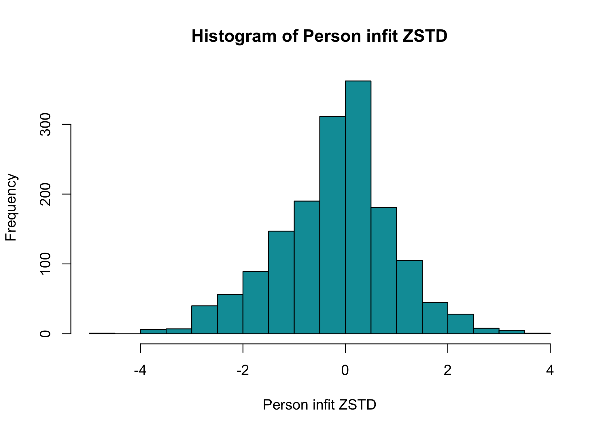
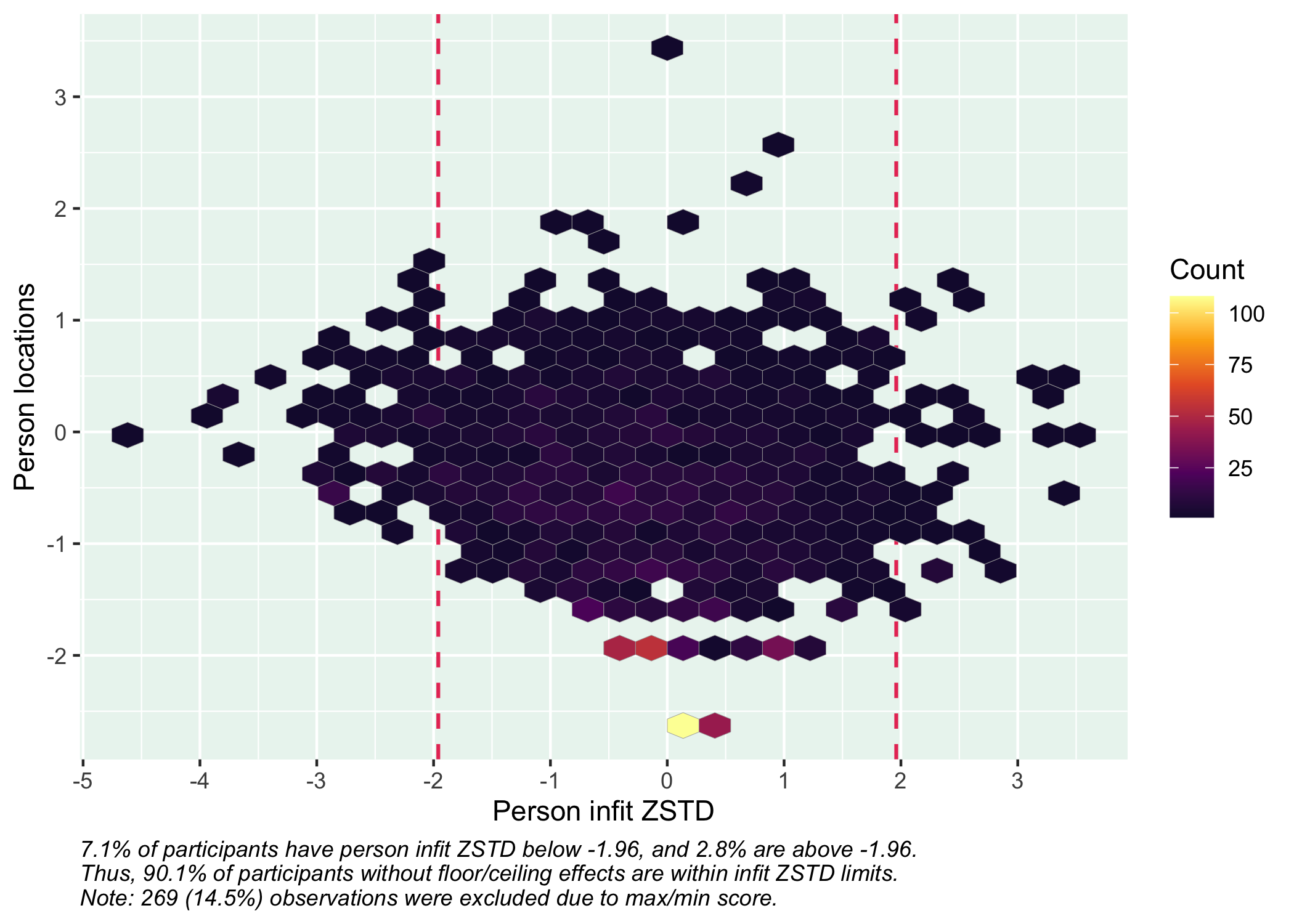
## Person fit
We can also look at how the respondents fit the Rasch model with these items. By default, `RIpfit()` outputs a histogram and a hex heatmap with the person infit ZSTD statistic, using +/- 1.96 as cutoff values. This is currently the only person fit method implemented in the `easyRasch` package, and the curious analyst is suggested to look at the package [PerFit](https://www.rdocumentation.org/packages/PerFit/versions/1.4.6/topics/PerFit-package) for more tools.
```{r}
RIpfit(df)
```
You can export the person fit values to a new variable in the dataframe by specifying `output = "dataframe"`, or if you just want the row numbers for respondents with deviant infit values, `output = "rowid"`.
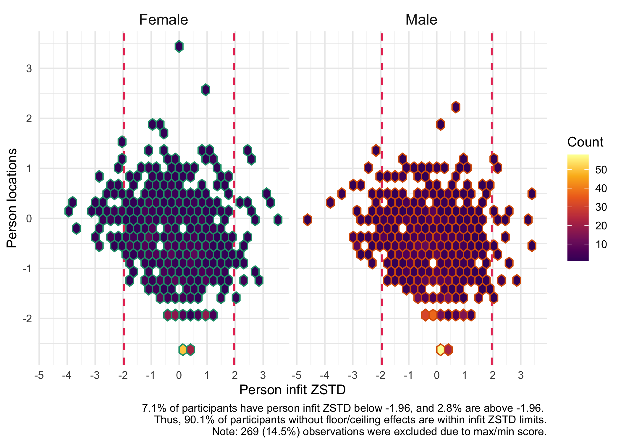
You can also specify a grouping variable to visualize the person fit for different groups.
```{r}
RIpfit(df, group = dif$Sex, output = "heatmap")
```
Person fit is a useful way to identify respondents with unexpected response patterns and investigate this further.
### `PerFit` sample code
::: {.callout-note icon="true"}
## Note
Since `easyRasch` 0.4.2.3, there is a new function: [`RIu3poly()`](https://pgmj.github.io/easyRasch/reference/RIu3poly.html). It will be added to the vignette later.
:::
While none of the functions in the `PerFit` package has been implemented in `easyRasch`, this is some code to get you started if you are interested in using it. There are multiple methods/functions available for polytomous and dichotomous data, see the package [documentation](https://www.rdocumentation.org/packages/PerFit/versions/1.4.6/topics/PerFit-package).
For this example, we'll use the non-parametric U3 statistic generalized to polytomous items [@emons_nonparametric_2008] and the smaller sample.
::: panel-tabset
#### U3poly
```{r}
library(PerFit)
pfit_u3poly <- U3poly(matrix = df500,
                      Ncat = 5, # make sure to input number of response categories, not thresholds
                      IRT.PModel = "PCM")
```
#### Cutoff information
```{r}
cutoff(pfit_u3poly)
```
#### Flagged respondents
```{r}
flagged.resp(pfit_u3poly) %>%
  pluck("Scores") %>%
  as.data.frame() %>%
  arrange(desc(PFscores))
```
:::
The dataframe shown under the tab `Flagged respondents` above contains a variable named `FlaggedID` which represents the row id's. This variable is useful if one wants to filter out respondents with deviant response patterns (person misfit). There are indications that persons with misfit may affect results of Andersen's LR-test for DIF [@artner_simulation_2016].
#### U3 poly considerations
It should be noted that `U3poly()` sometimes produces inconsistent results upon rerunning the same model, especially if you let it estimate the item and person parameters. For this reason, I have created a wrapper function that runs 100 iterations and returns the median percentage of misfitting individuals. You can review the code using `View(RIu3poly)` to see what the wrapper function is doing.
```{r}
RIu3poly(df500)
```
### Item fit without aberrant responses
We can remove the misfitting persons to see how that affects item fit. Let's also compare with the misfitting respondents identified by `RIpfit()`, also using the smaller sample.
```{r}
misfits <- flagged.resp(pfit_u3poly) %>%
  pluck("Scores") %>%
  as.data.frame() %>%
  pull(FlaggedID)

misfits2 <- RIpfit(df500, output = "rowid")
```
::: panel-tabset
#### All respondents
```{r}
RIitemfit(df500, simcut = simfit3)
```
#### U3 misfit removed
```{r}
RIitemfit(df500[-misfits,], simcut = simfit3)
```
#### ZSTD misfit removed
```{r}
RIitemfit(df500[-misfits2,], simcut = simfit3)
```
:::
## Item parameters
To allow others (and oneself) to use the item parameters estimated for estimation of person locations/thetas, we should make the item parameters available. The function will also write a csv-file with the item threshold locations. Estimations of person locations/thetas can be done with the `thetaEst()` function from the `catR` package. This is implemented in the function `RIestThetasOLD()`, see below for details.
First, we'll output the parameters into a table.
```{r}
RIitemparams(df)
```
The parameters can also be output to a dataframe or a file, using the option `output = "dataframe"` or `output = "file"`.
## Ordinal sum score to interval score
This table shows the corresponding "raw" ordinal sum score values and logit scores, with standard errors for each logit value. Interval scores are estimated using WL based on a simulated dataset using the item parameters estimated from the input dataset. The choice of WL as default is due to the lower bias compared to ML estimation [@warm1989;@kreiner_specific_2025].
(An option will hopefully be added at some point to create this table based on only item parameters.)
```{r}
RIscoreSE(df)
```
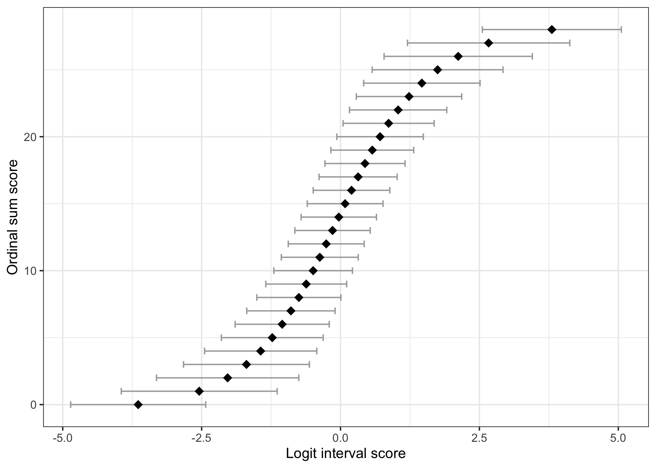
### Ordinal/interval figure
The figure below can also be generated to illustrate the relationship between ordinal sum score and logit interval score. The errorbars default to show the standard error at each point, multiplied by 1.96.
```{r}
RIscoreSE(df, output = "figure")
```
### Estimating interval level person scores
Based on the Rasch analysis output of item parameters, we can estimate each individuals location or score (also known as "theta"). `RIestThetas()` estimates item parameters from a partial credit model (PCM) and as default uses WL estimation [@warm1989;@kreiner_specific_2025] to output a dataframe with person locations and their measurement error (SEM) on the logit scale. However, this function is only appropriate if you have complete response data for all participants. If you have partial missingness, you need to use either `RIestThetasOLD()` or `RIestThetasCATr()`.
```{r}
thetas <- RIestThetas(df)

head(thetas)
```
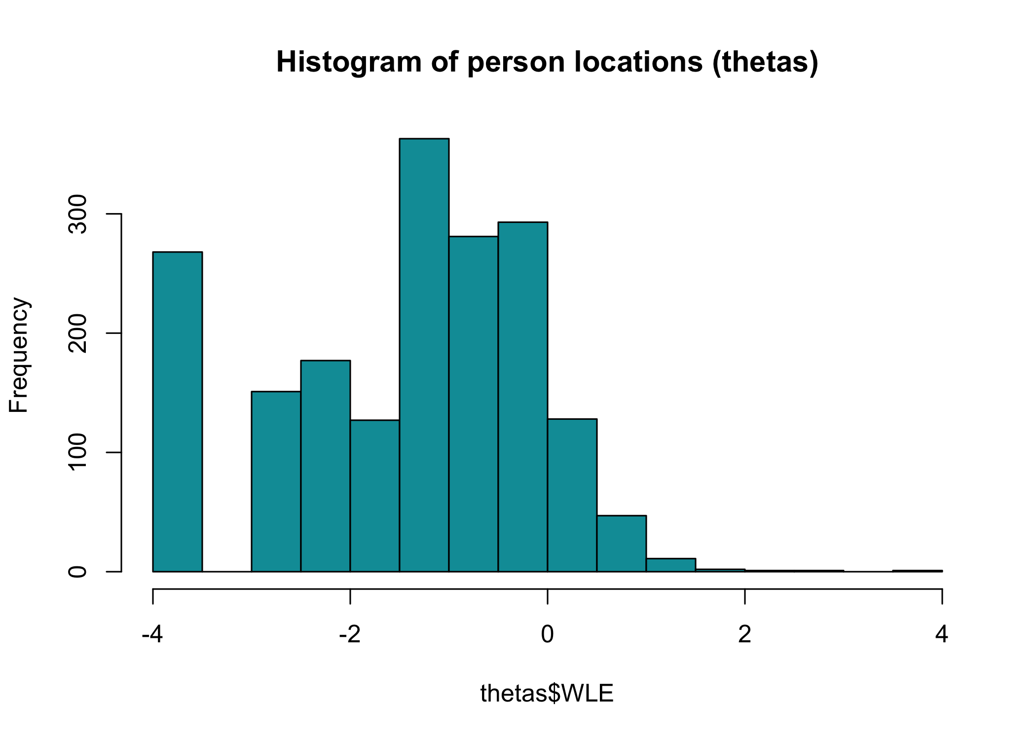
Each individual has a standard error of measurement (SEM) associated with their estimated location/score. This is included in the output of the `RIestThetas()` function as the `SEM` variable, as seen above. We can review the distribution of measurement error with a figure.
We can take a look at the distribution of person locations (thetas) using a histogram.
```{r}
hist(thetas$WLE,
     col = "#009ca6",
     main = "Histogram of person locations (thetas)",
     breaks = 20)
```
`RIestThetasOLD()` and `RIestThetasCATr()` can be used with a pre-specified item (threshold) location matrix.
If you would like to use an existing item threshold location matrix, this code may be helpful:
```{r}
itemParameters <- read_csv("itemParameters.csv") %>%
  as.matrix()
itemParameters
```
As you can see, this is a matrix object (not a dataframe), with each item as a row, and the threshold locations as columns.
## Figure design
Most of the figures created by the functions can be styled (colors, fonts, etc) by adding theme settings to them. You can use the standard ggplot function `theme()` and related theme-functions. As usual it is possible to "stack" theme functions, as seen in the example below.
You can also change coloring, axis limits/breaks, etc, just by adding ggplot options with a `+` sign.
A custom theme function, `theme_rise()`, is included in the `easyRasch` package. It might be easier to use if you are not familiar with `theme()`.
For instance, you might like to change the font to "Lato" for the item hierarchy figure, and make the background transparent.
```{r}
RIitemHierarchy(df) +
  theme_minimal() + # first apply the minimal theme to make the background transparent
  theme_rise(fontfamily = "Lato") # then apply theme_rise, which simplifies making changes to all plot elements
```
As of package version 0.1.30.0, the `RItargeting()` function allows more flexibility in styling too, by having an option to return a list object with the three separate plots. See the [NEWS](https://github.com/pgmj/easyRasch/blob/main/NEWS.md#01300) file for more details. Since the `RItargeting()` function uses the `patchwork` library to combine plots, you can also make use of [the many functions that `patchwork` includes](https://patchwork.data-imaginist.com/articles/patchwork.html). For instance, you can set a title with a specific theme:
``` {r}
RItargeting(df) + plot_annotation(title = "Targeting", theme = theme_rise(fontfamily = "Arial"))
```
In order to change font for text *inside* plots (such as "t1" for thresholds) you will need to add an additional line of code.
``` r
update_geom_defaults("text", list(family = "Lato"))
```
Please note that the line of code above updates the default settings for `geom_text()` for the whole session. Also, some functions, such as `RIloadLoc()`, make use of `geom_text_repel()`, for which you would need to change the code above from "text" to "text_repel".
A simple way to only change font family and font size would be to use `theme_minimal(base_family = "Calibri", base_size = 14)`. Please see the [reference page](https://ggplot2.tidyverse.org/reference/ggtheme.html) for default ggplot themes for alternatives to `theme_minimal()`.
## Software used {#sec-grateful}
The `grateful` package is a nice way to give credit to the packages used in making the analysis. The package can create both a bibliography file and a table object, which is handy for automatically creating a reference list based on the packages used (or at least explicitly loaded).
```{r}
library(grateful)
pkgs <- cite_packages(cite.tidyverse = TRUE,
                      output = "table",
                      bib.file = "grateful-refs.bib",
                      include.RStudio = FALSE,
                      out.dir = getwd())
# If kbl() is used to generate this table, the references will not be added to the Reference list.
formattable(pkgs,
            table.attr = 'class=\"table table-striped\" style="font-size: 13px; font-family: Lato; width: 80%"')
```
## Additional credits
Thanks to my [colleagues at RISE](https://www.ri.se/en/what-we-do/projects/center-for-category-based-measurements) for providing feedback and testing the package on Windows and MacOS platforms. Also, thanks to [Mike Linacre](https://www.winsteps.com/linacre.htm) and [Jeanette Melin](https://www.ri.se/en/person/jeanette-melin) for providing useful feedback to improve this vignette.
## Session info
```{r}
sessionInfo()
```
## References