We frequently use questionnaires to measure latent variables based on multiple items/indicators, but the connection between item responses and a latent trait score is often unclear. Here, I will present a way to visualize item responses and their corresponding latent score and measurement uncertainty that hopefully makes what lies behind the latent score much easier to understand.
It should be noted that the term “latent trait score” is not entirely established. The intent is to refer to what in Item Response Theory and Rasch modeling is labelled “theta” - 𝜃 (also known as “person ability”, “person location”, or “person score”). For each participant, IRT/Rasch models make it possible to both estimate a latent trait score on an interval scale and a measurement error specific for each participant’s score. The measurement error depends on the item properties and is not a constant value that is the same for all participants/scores.
In classical test theory, latent trait scores may be estimated using factor analysis and used in structural equation models. However, I have never seen anyone “export” the actual latent trait scores for each participant in a dataset, based on a confirmatory factor analysis (CFA). What is usually done, based on classical test theory/CFA, is to use the raw ordinal sum score as a representation of the latent variable.
Jump ahead to Section 5 to see the visualization and skip the psychometric background.
1 Background
The Mental Health Continuum Short Form (Ryff, 1989; Ryff, 2014) will be used as an example. I have conducted a Rasch analysis and preliminary results indicate that some modifications are needed for the response categories, and some items need to be removed. This will be reported elsewhere in greater detail. Here, only a summary of the changes and the measurement properties of the final set of items will be reported.
The analysis makes use of my R package for Rasch psychometric analysis, which in turn depends on (and automatically loads) a lot of packages. See the RISEkbmRasch vignette and GitHub package repository for more details.
Code
library(RISEkbmRasch)library(arrow)library(ggdist)library(ggpp)### some commands exist in multiple packages, here we define preferred ones that are frequently usedselect<-dplyr::selectcount<-dplyr::countrecode<-car::recoderename<-dplyr::rename# import item informationitemlabels<-read_excel("/Volumes/magnuspjo/RegionUppsala/data/RegUaItemlabelsEng.xls", sheet =1)%>%filter(str_detect(itemnr,"mhc"))itemresponses<-read_excel("/Volumes/magnuspjo/RegionUppsala/data/RegUaItemlabelsEng.xls", sheet =3)%>%rename(`How often during the past month did you feel...` =item)# import recoded datadf.all<-read_parquet("/Volumes/magnuspjo/RegionUppsala/data/RegUaLHUdata.parquet")df<-df.all# recode response categories to numericsdf<-df%>%mutate(across(starts_with("I1_"), ~recode(.x,"'Aldrig'=0; 'En eller två gånger'=1; '1 gång/vecka'=2; '2-3 gånger/vecka'=3; 'Nästan dagligen'=4; 'Dagligen'=5", as.factor =FALSE)))df<-df%>%filter(inars%in%c(2019,2021))%>%mutate(Age =recode(arskurs,"1='13 yo';2='15 yo';3=' 17 yo';9=NA;99=NA", as.factor =TRUE), Gender =recode(kon,"99=NA;9=NA;2='Girls';1='Boys'", as.factor =T),)%>%filter(Age%in%c("15 yo","17 yo"))%>%select(starts_with("I1_"),Age,Gender)%>%na.omit()# create variables for analysis of Differential Item Functioningdif.age<-df$Agedif.gender<-df$Genderdf$Age<-NULLdf$Gender<-NULL# set variable names to matchnames(df)<-itemlabels$itemnr
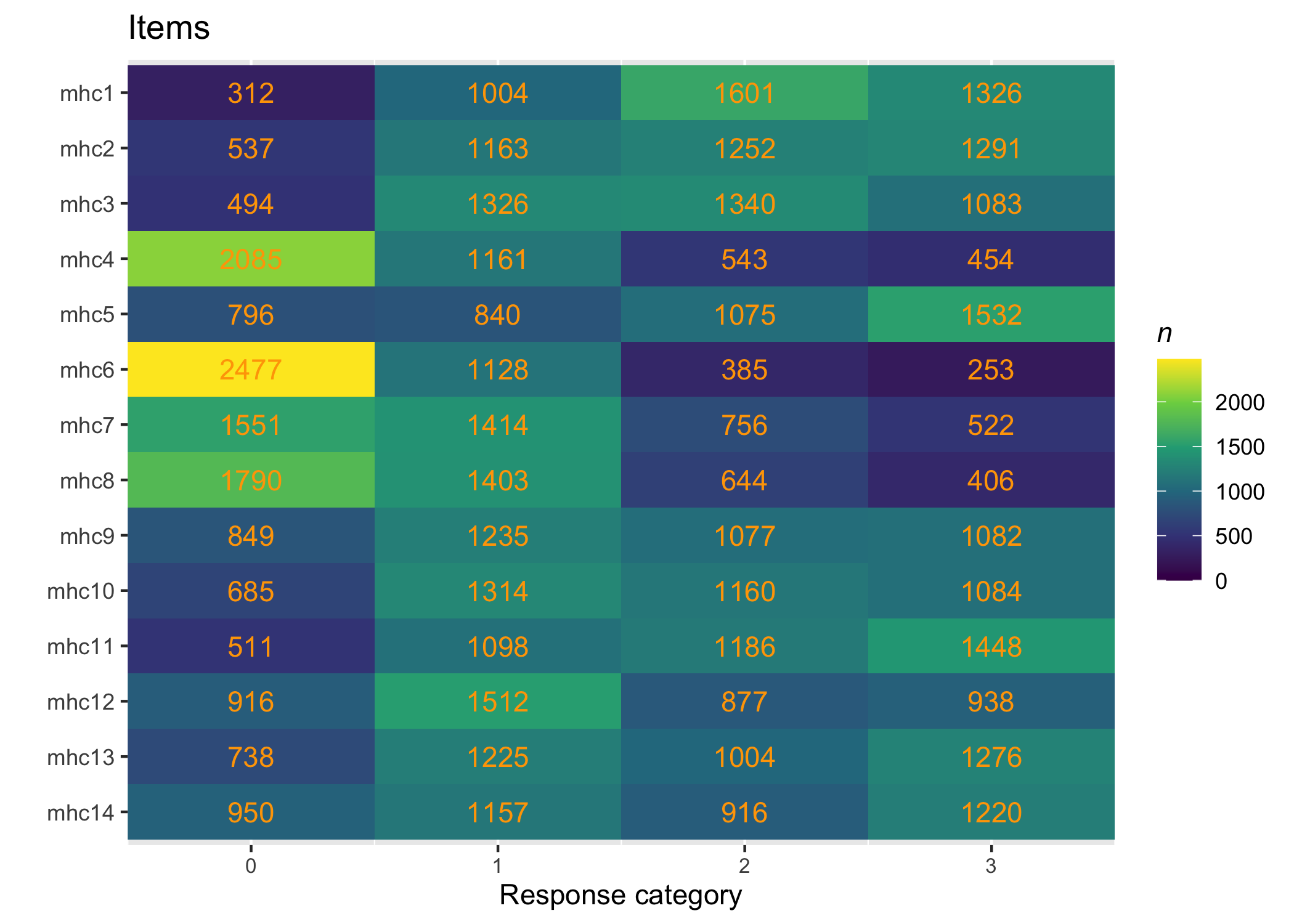
Questions in the MHC-SF are prefixed with How often during the past month did you feel…, and the items are listed below in Section 2 in the right-hand side margin.
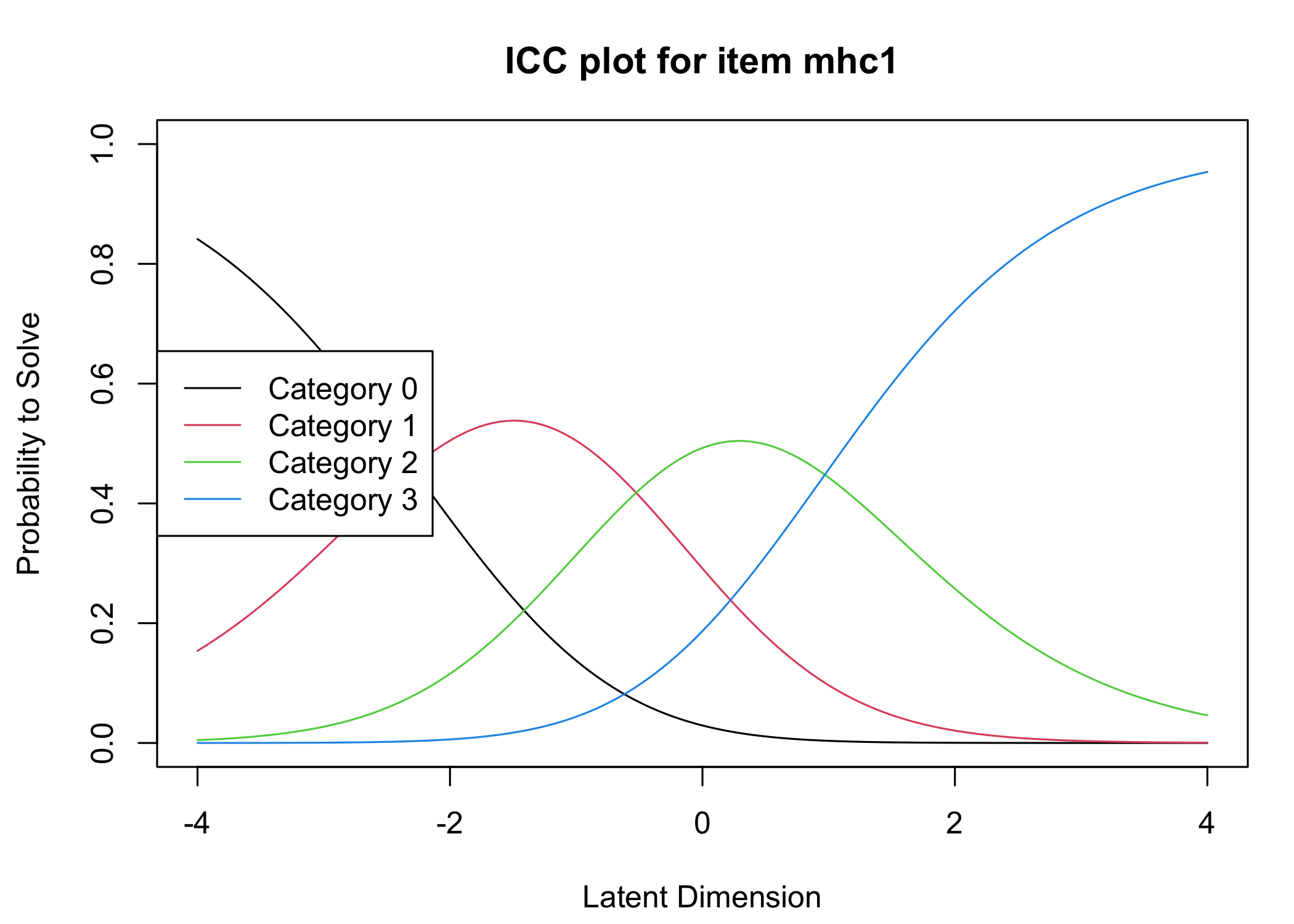
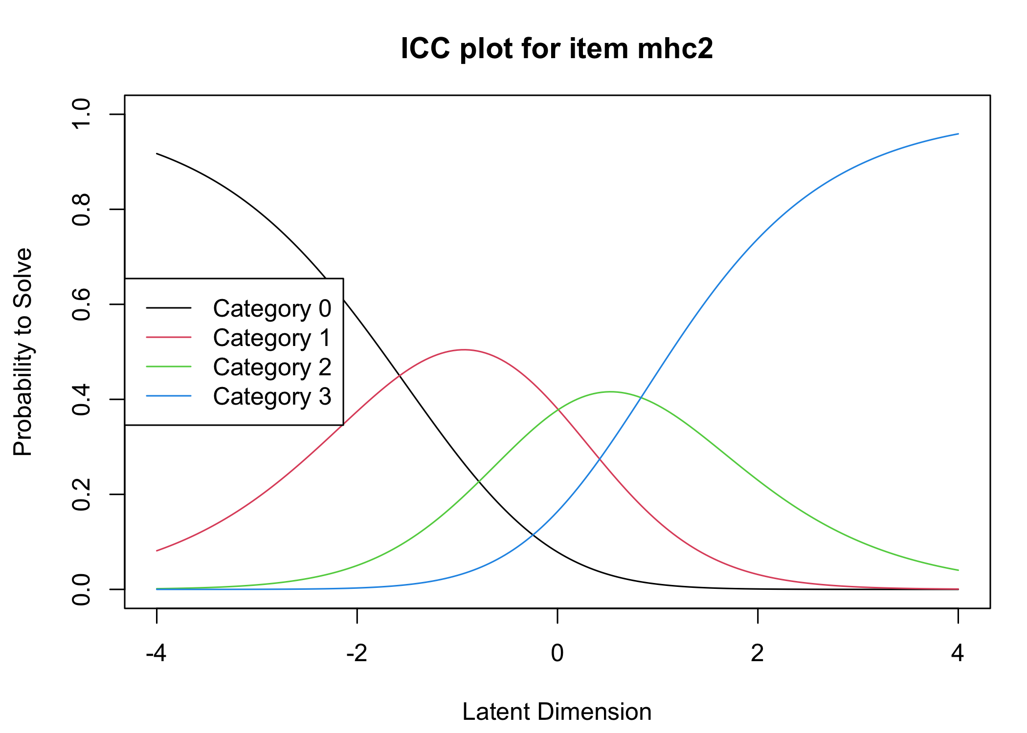
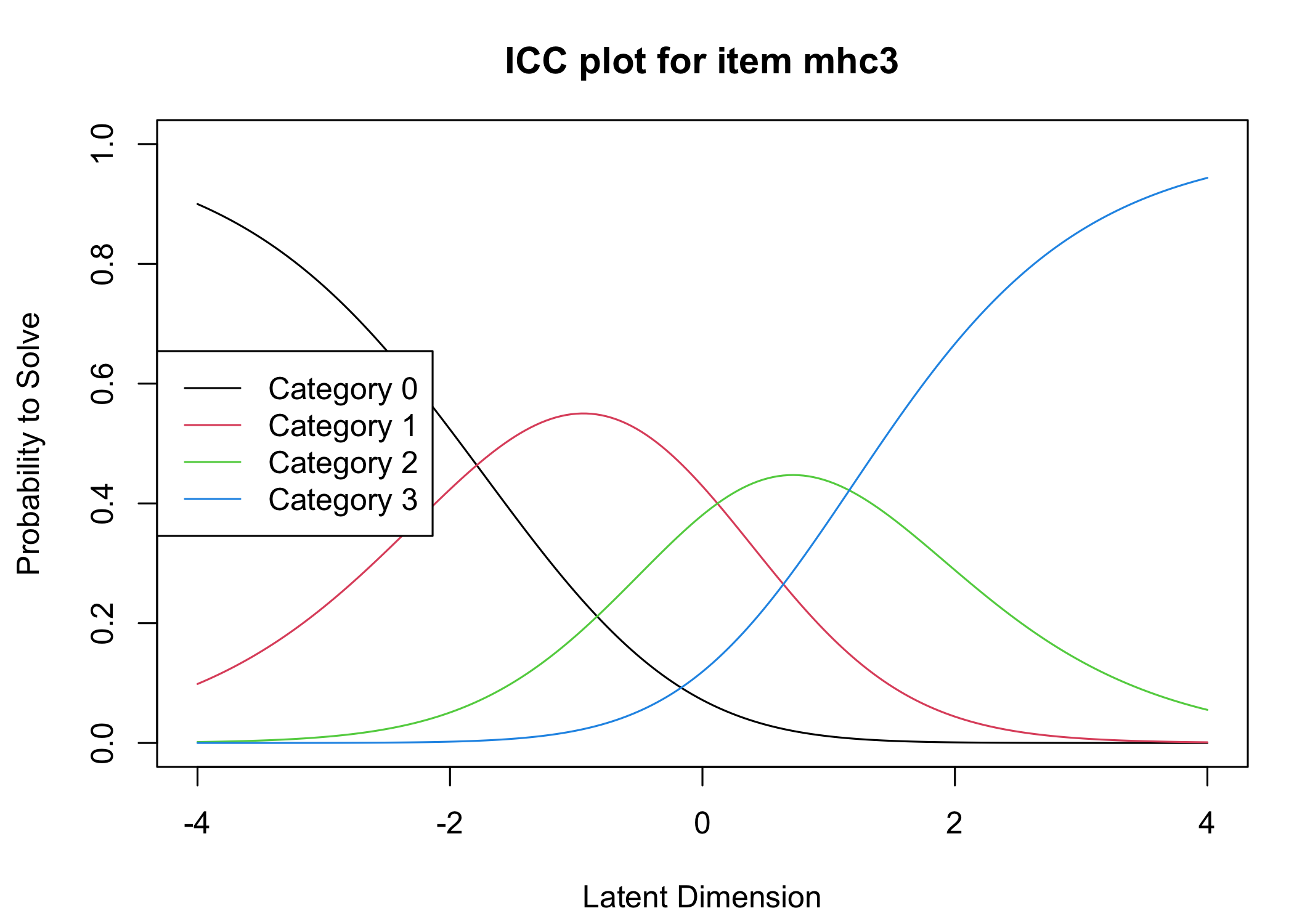
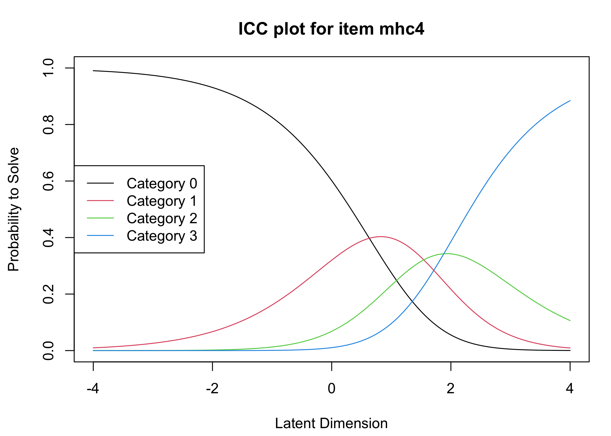
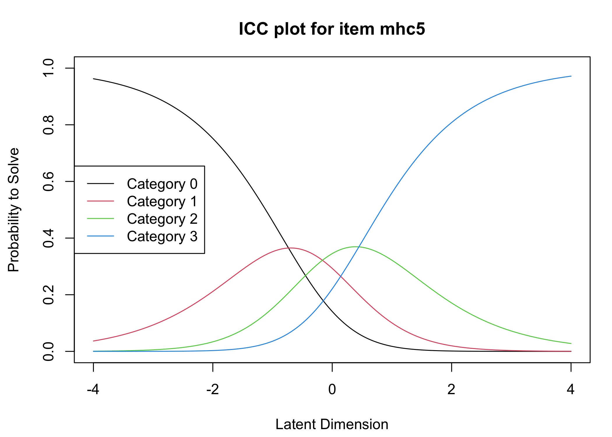
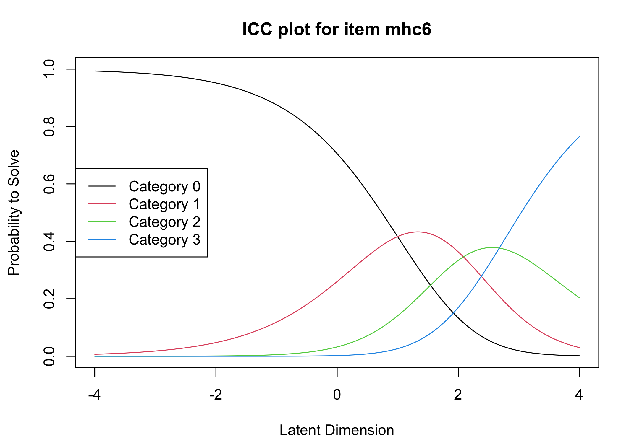
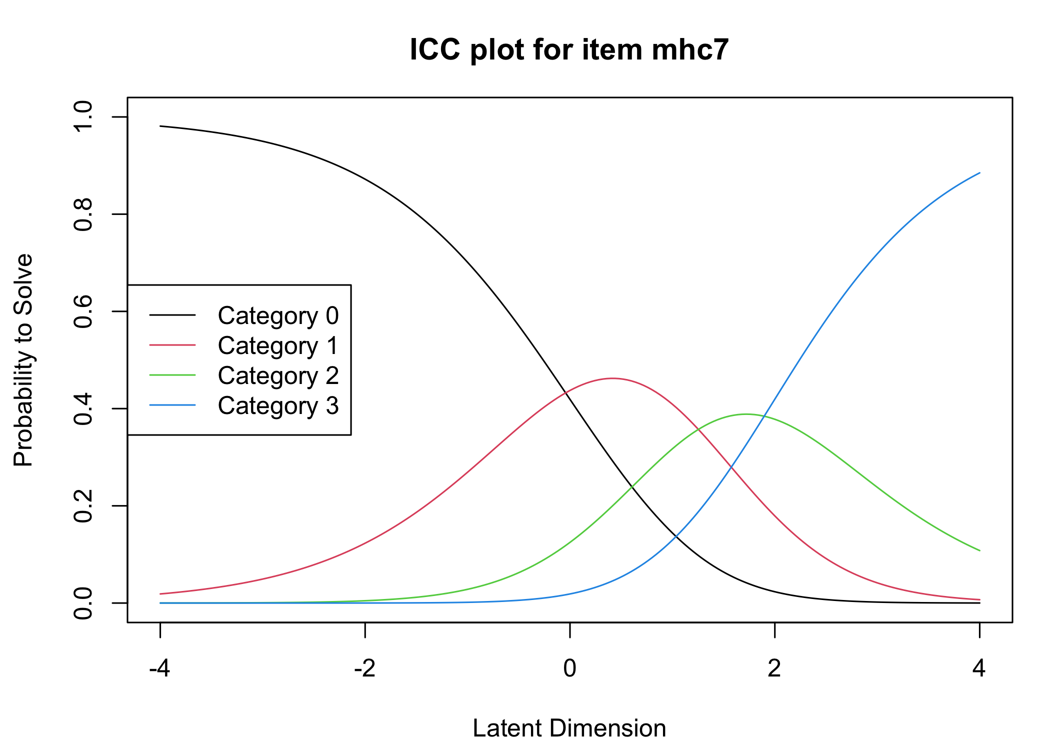
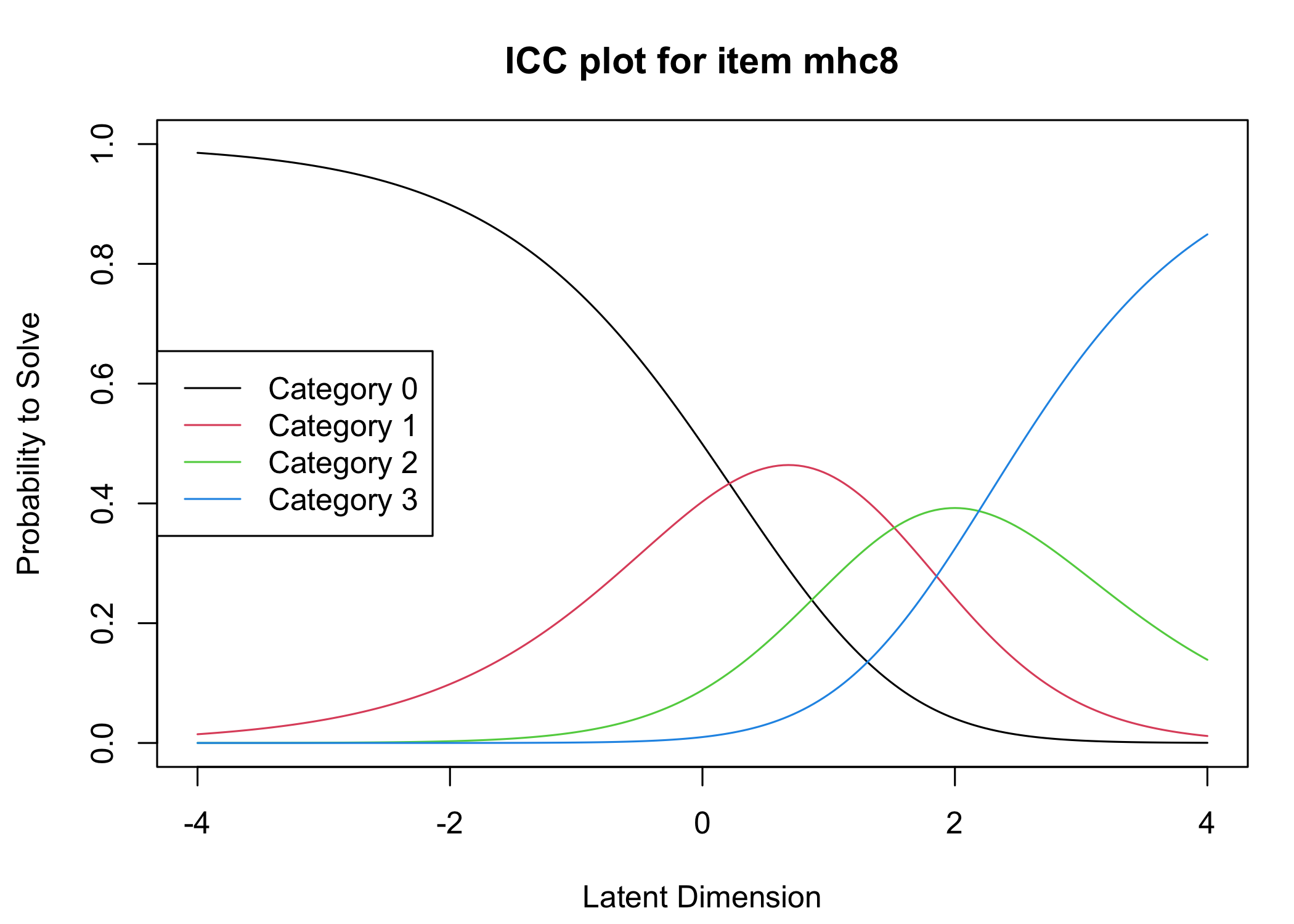
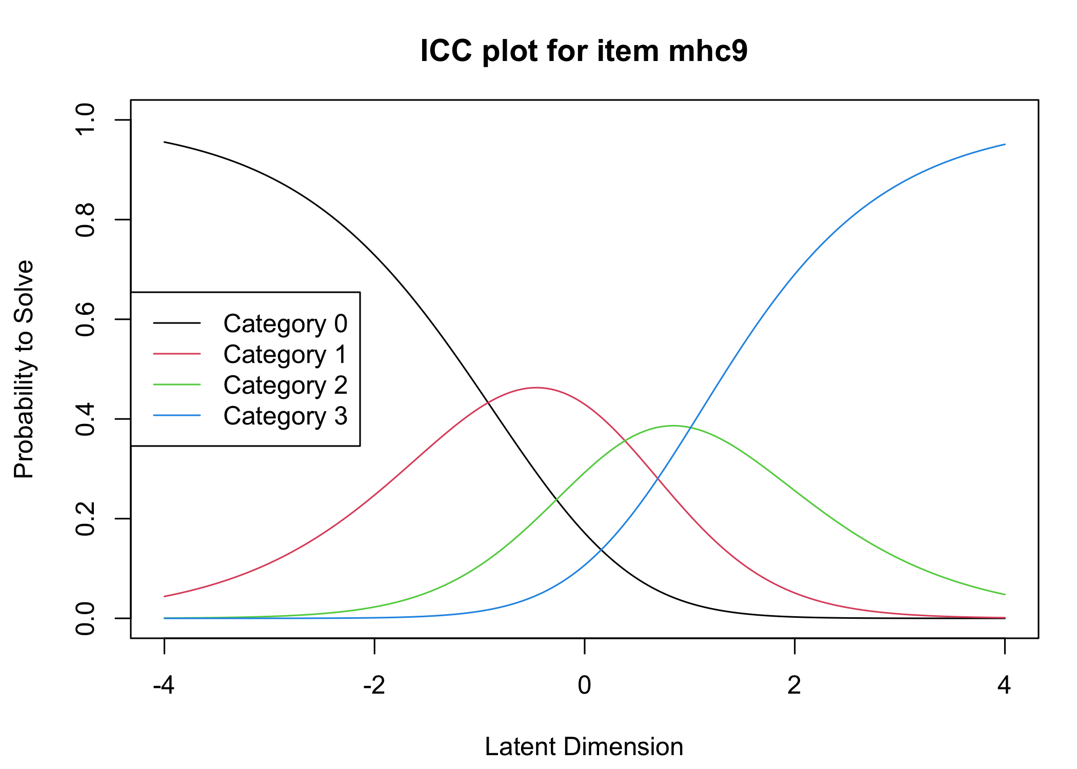
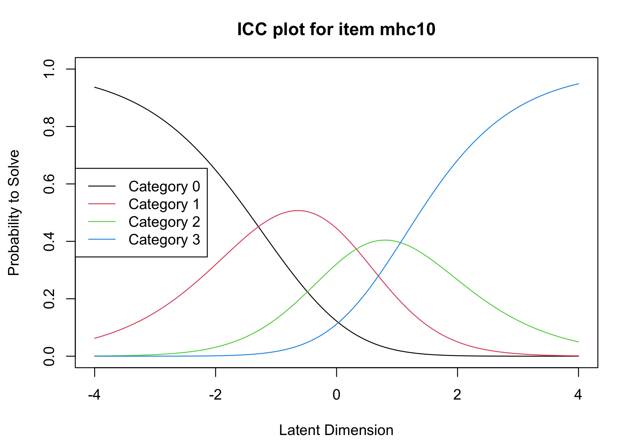
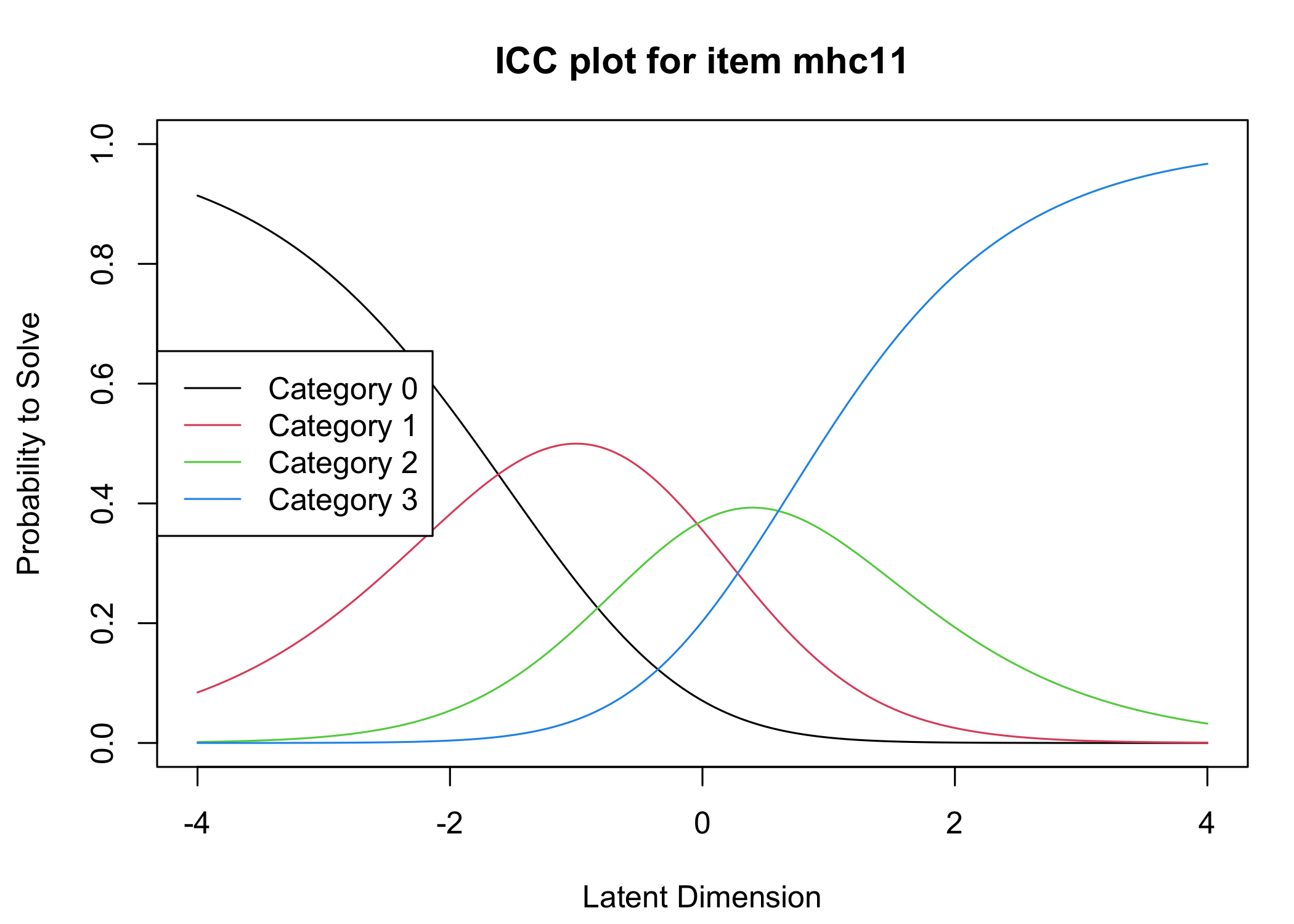
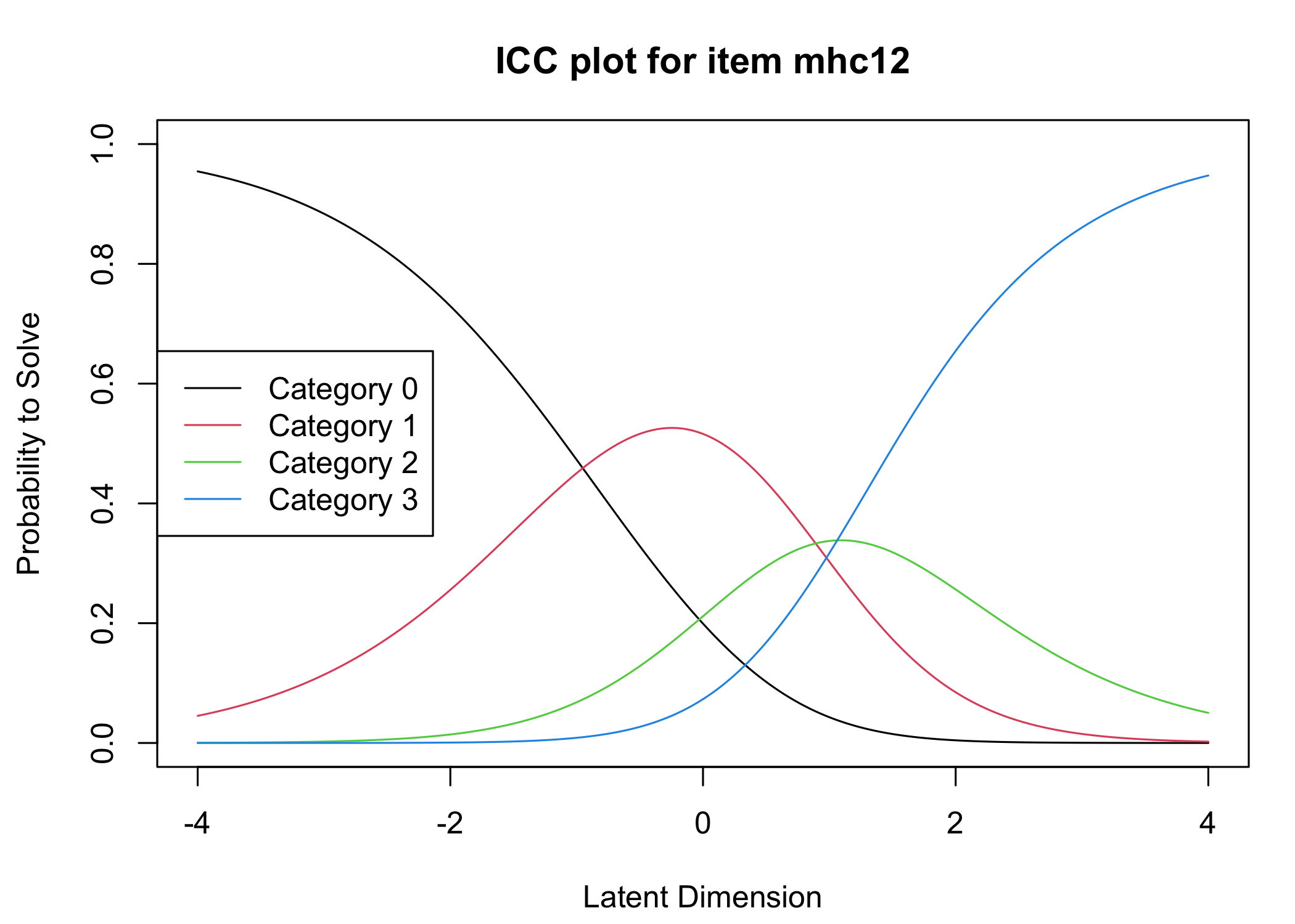
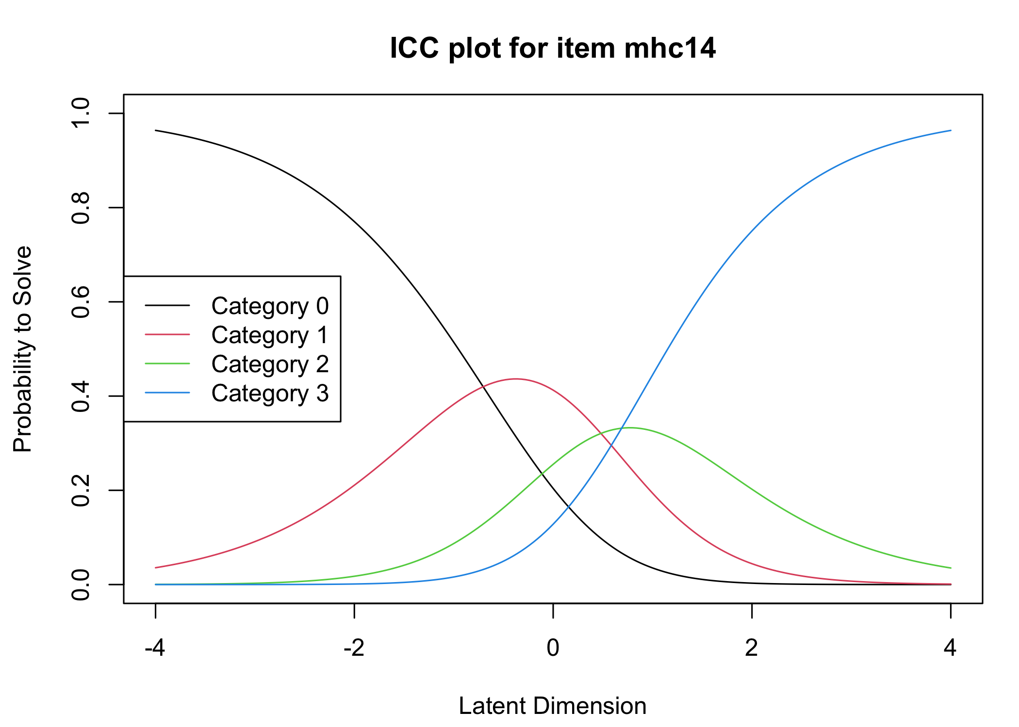
Six response categories were used, as specified in the original MHC-SF: every day, almost every day, about 2 or 3 times a week, about once a week, once or twice, never and the Rasch analysis found them disordered for all items. This means that some response categories do not contribute meaningful differential information to the latent score, compared to an adjacent response category - the categories are too similar to the respondents. After merging never with once or twice, and about once a week with about 2 or 3 times a week, the disordering was resolved. However, there are still quite small distances between item category thresholds, as shown in the ICC plots. This leaves us with 4 response categories for each item.
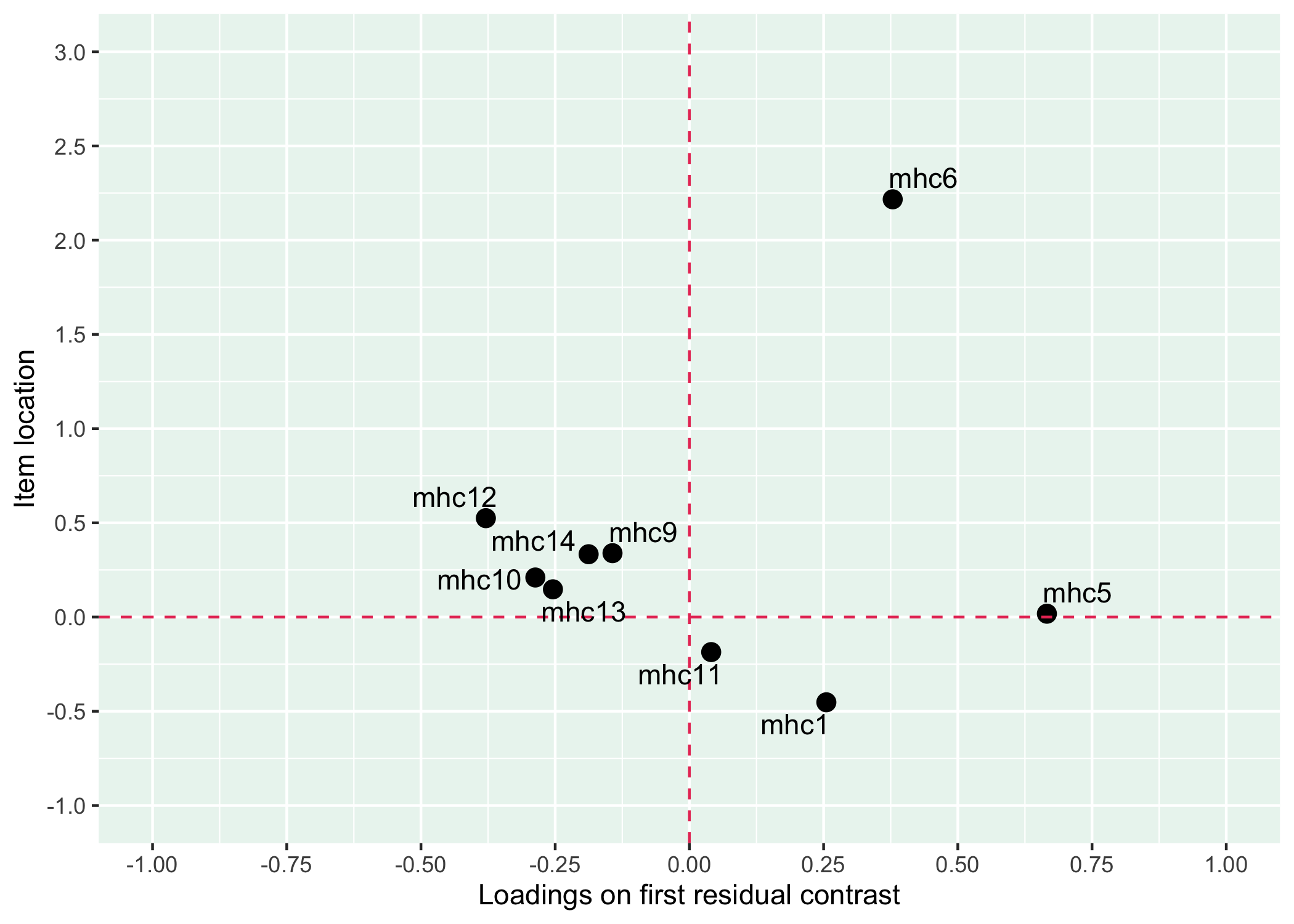
Five items were removed, mostly due to issues of multidimensionality and large residual correlations. Here, the analysis of remaining items is presented.
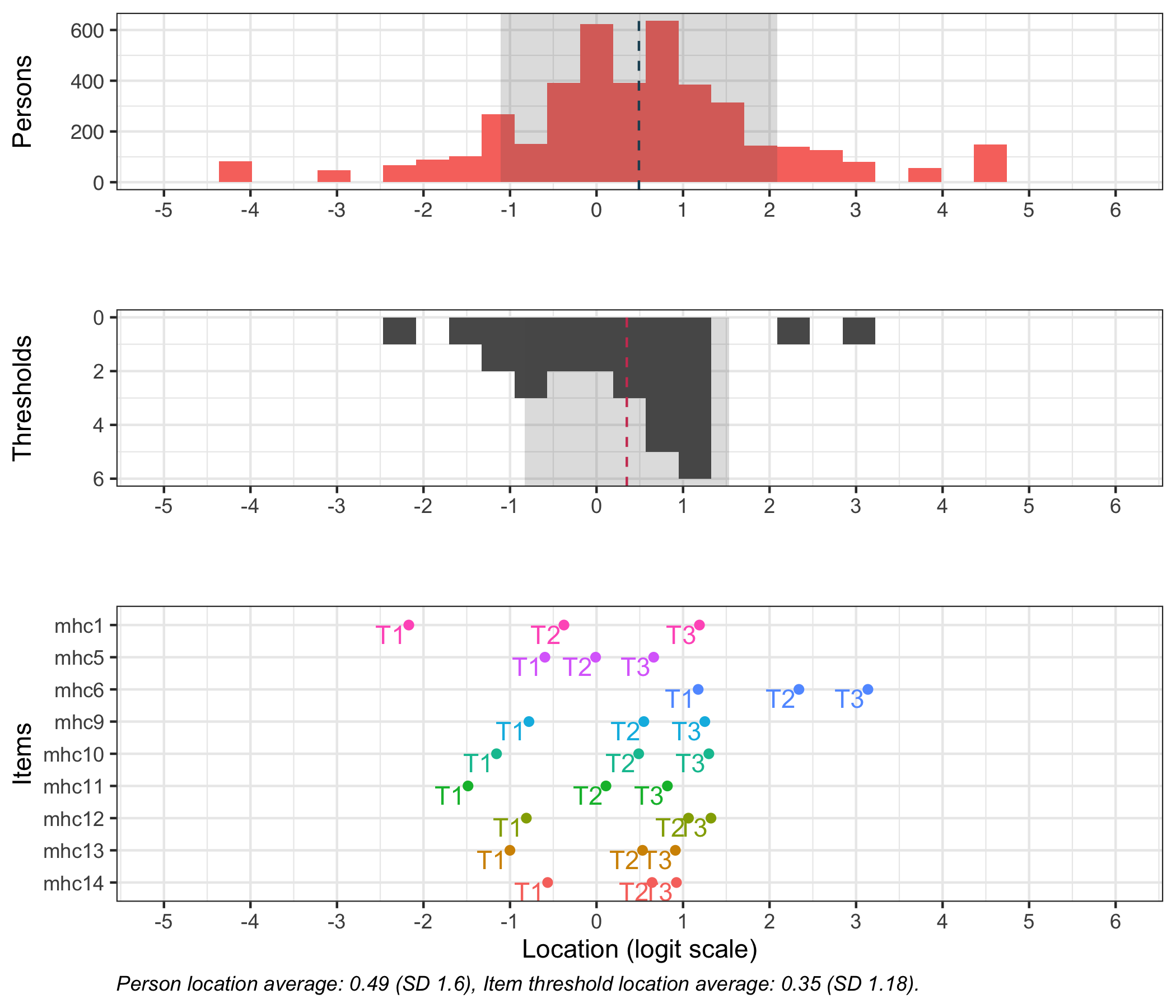
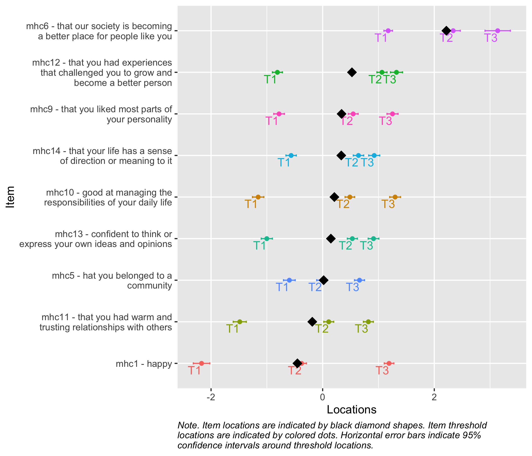
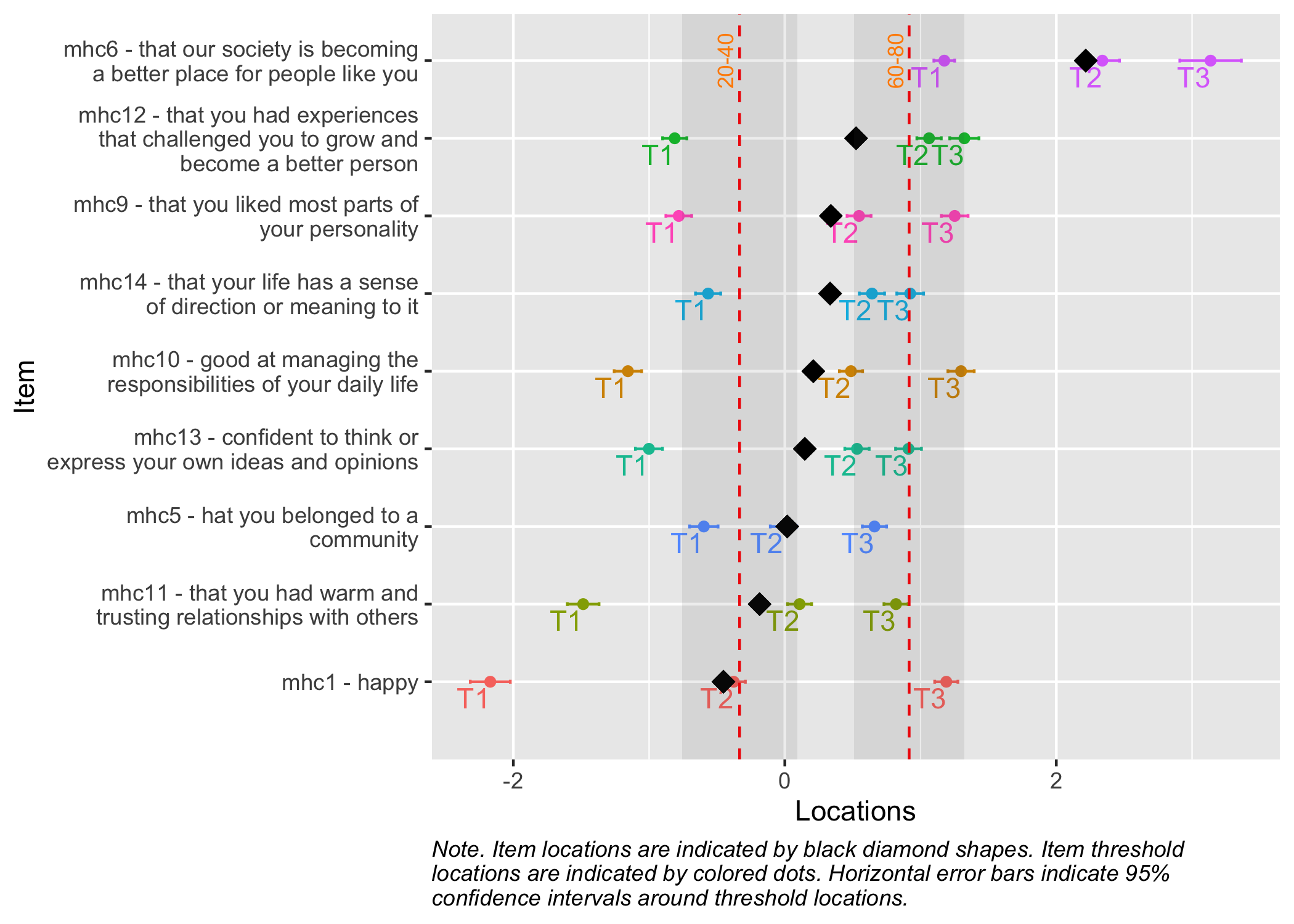
Item fit shows some minor issues, but we’ll leave them as good enough for the primary goal of visualization. Do have a look at the item hierarchy and give it some thought?
3 Estimating latent scores
First, we need the item threshold locations to later estimate person scores.
Actually, the function used to estimate person scores can automatically estimate the item parameters. But since this is just a practical use case, and you might be interested in applying the item parameters on your own dataset (since I cannot share this data), I thought it worth mentioning and displaying the parameters.
Code
df$MHCscore<-RIestThetas2(df, itemParams =MHCitemParameters, cpu =8)
Now we find the mode responses for each item based on the respondents in each quintile.
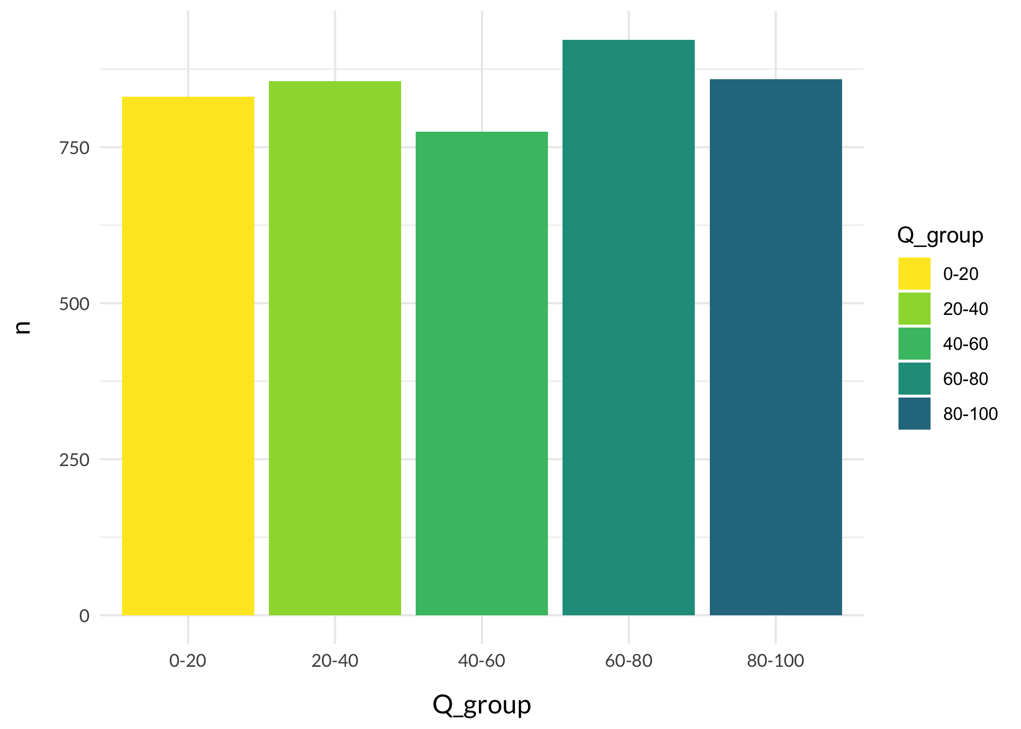
First, lets make groupings based on the quintile cutoff values.
Code
df<-df%>%mutate(Q_group =case_when(MHCscore<quintiles[1]~"0-20",MHCscore>=quintiles[1]&MHCscore<quintiles[2]~"20-40",MHCscore>=quintiles[2]&MHCscore<quintiles[3]~"40-60",MHCscore>=quintiles[3]&MHCscore<quintiles[4]~"60-80",MHCscore>=quintiles[4]~"80-100",TRUE~NA))df%>%count(Q_group)%>%ggplot(aes(x =Q_group, y =n, fill =Q_group))+geom_col()+scale_fill_viridis_d(begin =0.4, direction =-1)+theme_minimal()+theme_rise()
Identifying mode response categories for each item for each group is the next step
Estimating the latent score and SEM for each group’s mode response pattern.
Code
# sorry for the copy+paste code here...avg1<-thetaEst(MHCitemParameters, modeResponses$V1, model ="PCM", method ="WL")sem1<-semTheta(thEst =avg1, it =MHCitemParameters, x =modeResponses$V1, model ="PCM", method ="WL")avg2<-thetaEst(MHCitemParameters, modeResponses$V2, model ="PCM", method ="WL")sem2<-semTheta(thEst =avg2, it =MHCitemParameters, x =modeResponses$V2, model ="PCM", method ="WL")avg3<-thetaEst(MHCitemParameters, modeResponses$V3, model ="PCM", method ="WL")sem3<-semTheta(thEst =avg3, it =MHCitemParameters, x =modeResponses$V3, model ="PCM", method ="WL")avg4<-thetaEst(MHCitemParameters, modeResponses$V4, model ="PCM", method ="WL")sem4<-semTheta(thEst =avg4, it =MHCitemParameters, x =modeResponses$V4, model ="PCM", method ="WL")avg5<-thetaEst(MHCitemParameters, modeResponses$V5, model ="PCM", method ="WL")sem5<-semTheta(thEst =avg5, it =MHCitemParameters, x =modeResponses$V5, model ="PCM", method ="WL")
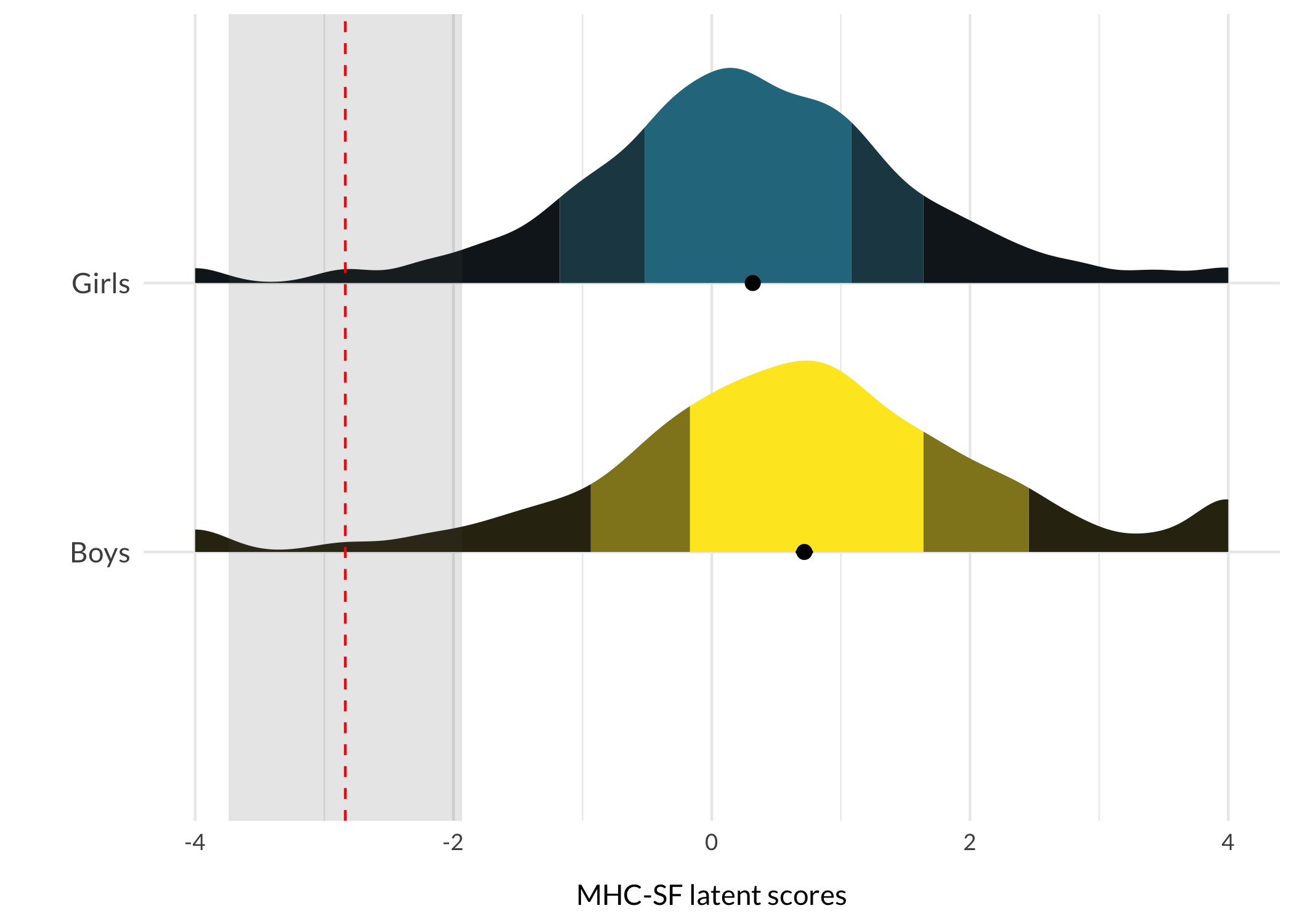
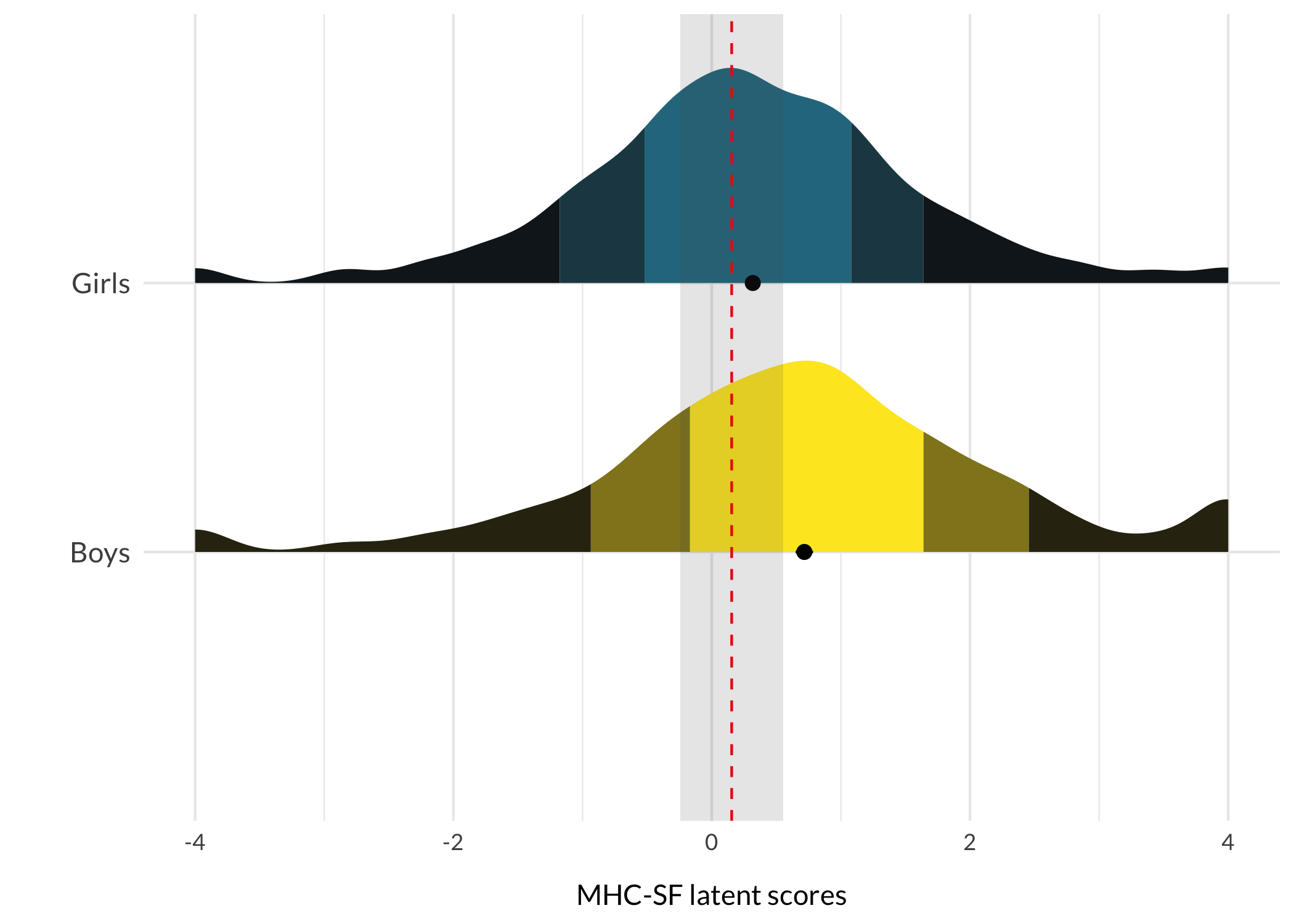
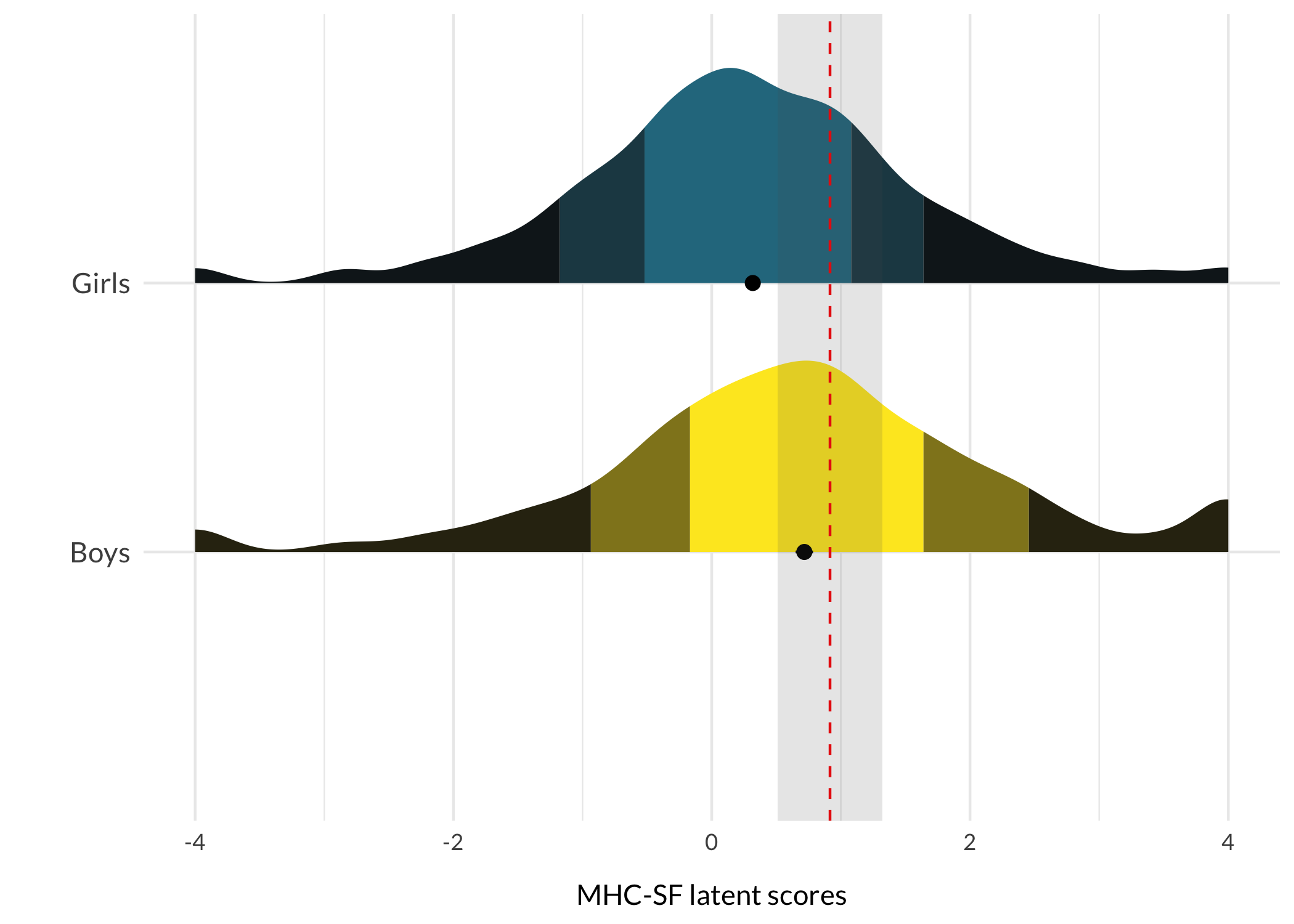
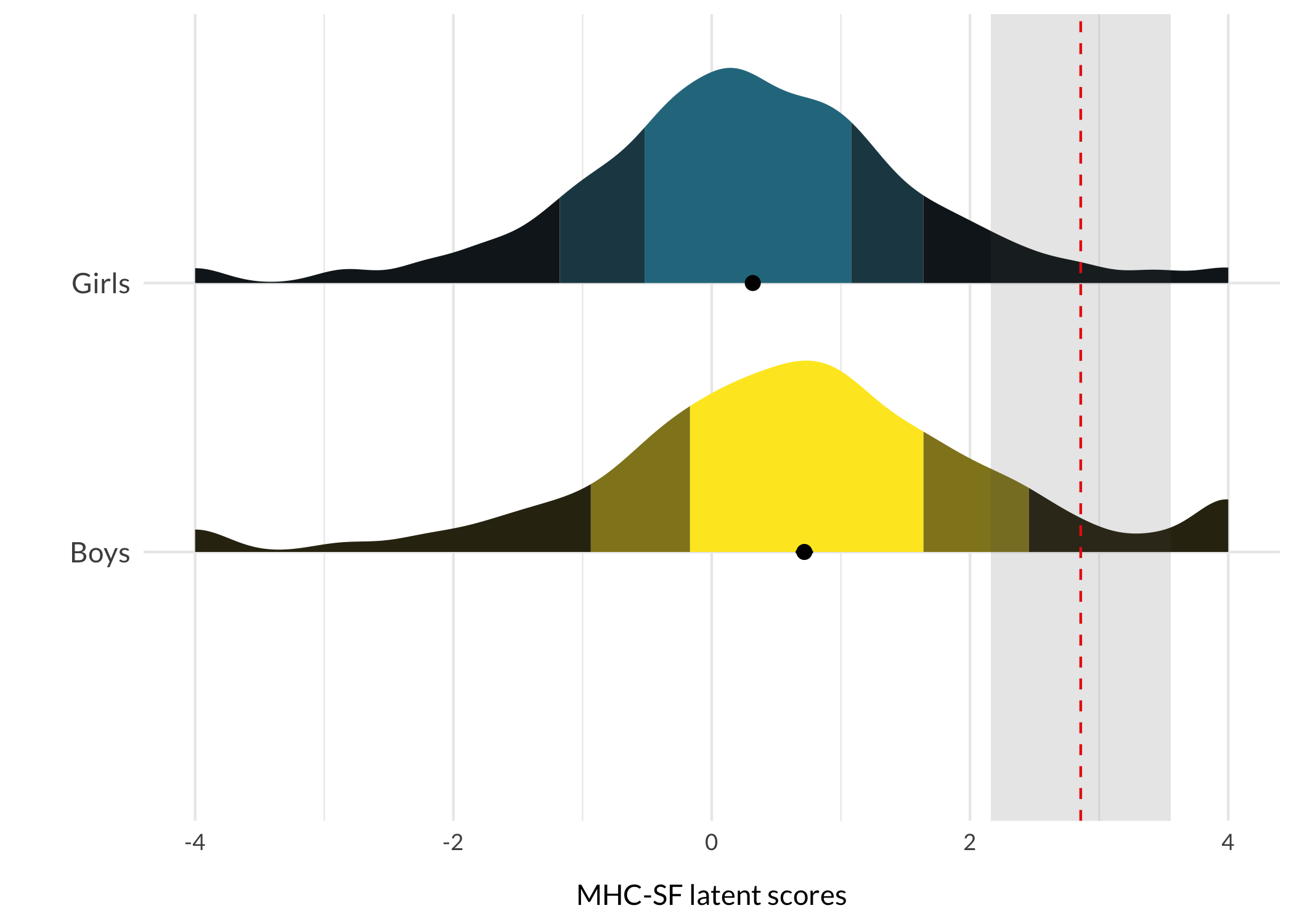
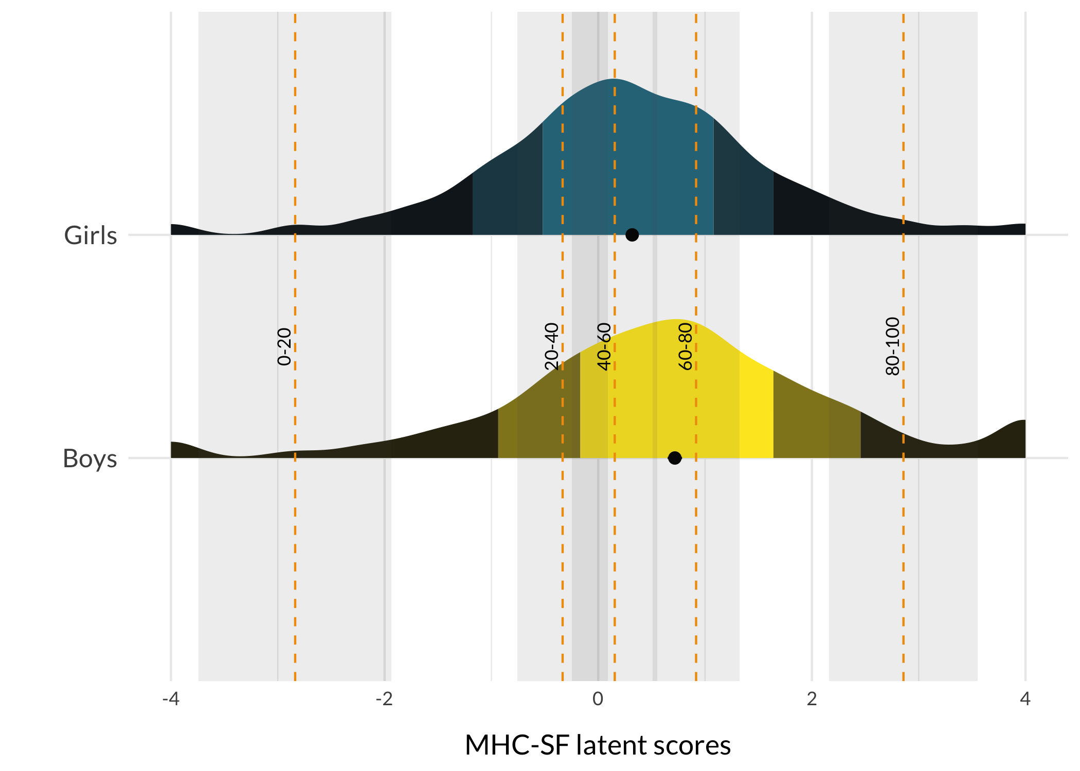
5 Visualization
Code
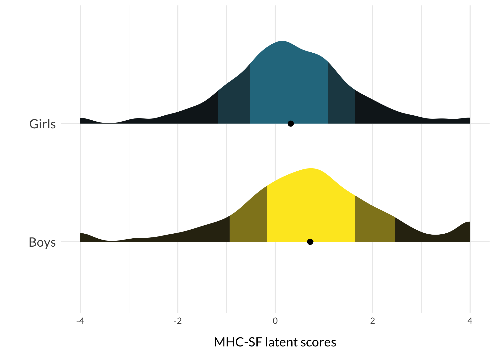
respTable<-function(qLevel){# typical response patterns for different risk levelsif(qLevel=="0-20"){p.resp<-modeResponses$V1}elseif(qLevel=="20-40"){p.resp<-modeResponses$V2}elseif(qLevel=="40-60"){p.resp<-modeResponses$V3}elseif(qLevel=="60-80"){p.resp<-modeResponses$V4}elseif(qLevel=="80-100"){p.resp<-modeResponses$V5}itemresponses%>%formattable(., align =c("r", "l", "c", "c", "c", "c", "c"), list(formattable::area(row =1, col =3+p.resp[1])~color_tile("lightblue", "lightpink"),formattable::area(row =2, col =3+p.resp[2])~color_tile("lightblue", "lightpink"),formattable::area(row =3, col =3+p.resp[3])~color_tile("lightblue", "lightpink"),formattable::area(row =4, col =3+p.resp[4])~color_tile("lightblue", "lightpink"),formattable::area(row =5, col =3+p.resp[5])~color_tile("lightblue", "lightpink"),formattable::area(row =6, col =3+p.resp[6])~color_tile("lightblue", "lightpink"),formattable::area(row =7, col =3+p.resp[7])~color_tile("lightblue", "lightpink"),formattable::area(row =8, col =3+p.resp[8])~color_tile("lightblue", "lightpink"),formattable::area(row =9, col =3+p.resp[9])~color_tile("lightblue", "lightpink")), table.attr ='class=\"table table-striped\" style="font-size: 15px; font-family: Lato"')}respDist<-function(qLevel){if(qLevel=="0-20"){score<-avg1sem<-sem1}elseif(qLevel=="20-40"){score<-avg2sem<-sem2}elseif(qLevel=="40-60"){score<-avg3sem<-sem3}elseif(qLevel=="60-80"){score<-avg4sem<-sem4}elseif(qLevel=="80-100"){score<-avg5sem<-sem5}qlabel<-qLevelggplot(df, aes(x =MHCscore, y =Gender, fill =Gender))+stat_slab( side ="right", show.legend =F, scale =0.8, justification =0,aes(fill_ramp =after_stat(level)), .width =c(.50, .75, 1))+stat_summary( fun.data ="mean_cl_normal", show.legend =F, size =.4, position =position_dodge2nudge(x =.05, width =.8))+scale_fill_ramp_discrete(from ="black", aesthetics ="fill_ramp")+scale_fill_viridis_d(begin =0.4, direction =-1)+geom_vline(xintercept =score, color ="red", linetype =2)+annotate("rect", ymin =0, ymax =Inf, xmin =score-sem, xmax =score+sem, alpha =.15)+#annotate("text", label = qlabel, x = score-0.12, y = 1.5, # angle = 90, size = 4, family = "Lato") +xlab("MHC-SF latent scores")+ylab("")+theme_minimal()+theme_rise(axissize =11)+theme(axis.text.y =element_text(size =11))+scale_y_discrete(expand =c(0,0))}
Allaire, J., Xie, Y., McPherson, J., Luraschi, J., Ushey, K., Atkins, A., Wickham, H., Cheng, J., Chang, W., & Iannone, R. (2023). Rmarkdown: Dynamic documents for r. https://github.com/rstudio/rmarkdown
Richardson, N., Cook, I., Crane, N., Dunnington, D., François, R., Keane, J., Moldovan-Grünfeld, D., Ooms, J., & Apache Arrow. (2022). Arrow: Integration to ’apache’ ’arrow’. https://CRAN.R-project.org/package=arrow
Rodríguez-Sánchez, F., Jackson, C. P., & Hutchins, S. D. (2022). Grateful: Facilitate citation of r packages. https://github.com/Pakillo/grateful
Ryff, C. D. (1989). Happiness Is Everything, or Is It? Explorations on the Meaning of Psychological Well-Being. Journal of Personality and Social Psychology, 57(6), 1069–1081. https://doi.org/http://dx.doi.org/10.1037/0022-3514.57.6.1069
Ryff, C. D. (2014). Psychological Well-Being Revisited: Advances in the Science and Practice of Eudaimonia. Psychotherapy and Psychosomatics, 83(1), 10–28. https://doi.org/10.1159/000353263
Wickham, H., Averick, M., Bryan, J., Chang, W., McGowan, L. D., François, R., Grolemund, G., Hayes, A., Henry, L., Hester, J., Kuhn, M., Pedersen, T. L., Miller, E., Bache, S. M., Müller, K., Ooms, J., Robinson, D., Seidel, D. P., Spinu, V., … Yutani, H. (2019). Welcome to the tidyverse. Journal of Open Source Software, 4(43), 1686. https://doi.org/10.21105/joss.01686
---title: "What's in a latent trait score?"author: name: Magnus Johansson affiliation: RISE Research Institutes of Sweden affiliation-url: https://www.ri.se/sv/vad-vi-gor/expertiser/kategoriskt-baserade-matningar orcid: 0000-0003-1669-592Xdate: 2023-02-24citation: type: 'webpage'csl: ../apa.cslgoogle-scholar: trueformat: html: code-fold: truewebsite: twitter-card: image: "https://pgmj.github.io/latentResp/LatentResponse_files/figure-html/unnamed-chunk-26-1.png"execute: cache: true warning: false message: falsebibliography:- references.bib- grateful-refs.bibeditor_options: chunk_output_type: console---We frequently use questionnaires to measure latent variables based on multiple items/indicators, but the connection between item responses and a latent trait score is often unclear. Here, I will present a way to visualize item responses and their corresponding latent score and measurement uncertainty that hopefully makes what lies behind the latent score much easier to understand.It should be noted that the term "latent trait score" is not entirely established. The intent is to refer to what in Item Response Theory and Rasch modeling is labelled "theta" - 𝜃 (also known as "person ability", "person location", or "person score"). For each participant, IRT/Rasch models make it possible to both estimate a latent trait score on an interval scale and a measurement error specific for each participant's score. The measurement error depends on the item properties and is not a constant value that is the same for all participants/scores.In classical test theory, latent trait scores may be estimated using factor analysis and used in structural equation models. However, I have never seen anyone "export" the actual latent trait scores for each participant in a dataset, based on a confirmatory factor analysis (CFA). What is usually done, based on classical test theory/CFA, is to use the raw ordinal sum score as a representation of the latent variable.Jump ahead to @sec-visualization to see the visualization and skip the psychometric background.## BackgroundThe Mental Health Continuum Short Form [@ryff1989; @ryff2014] will be used as an example. I have conducted a Rasch analysis and preliminary results indicate that some modifications are needed for the response categories, and some items need to be removed. This will be reported elsewhere in greater detail. Here, only a summary of the changes and the measurement properties of the final set of items will be reported.The analysis makes use of my R package for Rasch psychometric analysis, which in turn depends on (and automatically loads) a lot of packages. See the [RISEkbmRasch vignette](https://pgmj.github.io/raschrvignette/RaschRvign.html) and [GitHub package repository](https://github.com/pgmj/RISEkbmRasch) for more details.```{r}library(RISEkbmRasch)library(arrow)library(ggdist)library(ggpp)### some commands exist in multiple packages, here we define preferred ones that are frequently usedselect <- dplyr::selectcount <- dplyr::countrecode <- car::recoderename <- dplyr::rename# import item informationitemlabels <-read_excel("/Volumes/magnuspjo/RegionUppsala/data/RegUaItemlabelsEng.xls", sheet =1) %>%filter(str_detect(itemnr,"mhc"))itemresponses <-read_excel("/Volumes/magnuspjo/RegionUppsala/data/RegUaItemlabelsEng.xls", sheet =3) %>%rename(`How often during the past month did you feel...`= item)# import recoded datadf.all <-read_parquet("/Volumes/magnuspjo/RegionUppsala/data/RegUaLHUdata.parquet")df <- df.all# recode response categories to numericsdf <- df %>%mutate(across(starts_with("I1_"), ~recode(.x,"'Aldrig'=0; 'En eller två gånger'=1; '1 gång/vecka'=2; '2-3 gånger/vecka'=3; 'Nästan dagligen'=4; 'Dagligen'=5",as.factor =FALSE) ))df <- df %>%filter(inars %in%c(2019,2021)) %>%mutate(Age =recode(arskurs,"1='13 yo';2='15 yo';3=' 17 yo';9=NA;99=NA", as.factor =TRUE),Gender =recode(kon,"99=NA;9=NA;2='Girls';1='Boys'", as.factor = T), ) %>%filter(Age %in%c("15 yo","17 yo")) %>%select(starts_with("I1_"),Age,Gender) %>%na.omit()# create variables for analysis of Differential Item Functioningdif.age <- df$Agedif.gender <- df$Genderdf$Age <-NULLdf$Gender <-NULL# set variable names to matchnames(df) <- itemlabels$itemnr```Questions in the MHC-SF are prefixed with ***How often during the past month did you feel...***, and the items are listed below in @sec-rasch in the right-hand side margin.Six response categories were used, as specified in the original MHC-SF: ***every day, almost every day, about 2 or 3 times a week, about once a week, once or twice, never*** and the Rasch analysis found them disordered for all items. This means that some response categories do not contribute meaningful differential information to the latent score, compared to an adjacent response category - the categories are too similar to the respondents. After merging ***never*** with ***once or twice***, and ***about once a week*** with ***about 2 or 3 times a week***, the disordering was resolved. However, there are still quite small distances between item category thresholds, as shown in the ICC plots. This leaves us with 4 response categories for each item.The sample consists of `r nrow(df)` respondents.```{r}for (i in itemlabels$itemnr) { df[[i]] <-recode(df[[i]],"1=0;2=1;3=1;4=2;5=3",as.factor =FALSE)}```::: panel-tabset### Tileplot```{r}RItileplot(df)```### ICC plots```{r}#| layout-ncol: 3ermOut <-PCM(df)plotICC(ermOut)```:::## Rasch analysis summary {#sec-rasch}Five items were removed, mostly due to issues of multidimensionality and large residual correlations. Here, the analysis of remaining items is presented.```{r}removed.items <-c("mhc2","mhc3","mhc4","mhc8","mhc7")df <- df %>%select(!any_of(removed.items))``````{r}#| column: margin#| echo: falseRIlistItemsMargin(df, fontsize =12)```::: panel-tabset### Item fit```{r}RIitemfitPCM2(df, 300, 32, 8)```### PCA```{r}#| tbl-cap: "PCA of Rasch model residuals"RIpcmPCA(df)```### Residual correlations```{r}RIresidcorr(df, cutoff =0.2)```### 1st contrast loadings```{r}RIloadLoc(df)```### Targeting```{r}#| fig-height: 6# increase fig-height above as needed, if you have many itemsRItargeting(df)```### Item hierarchy```{r}#| fig-height: 6RIitemHierarchy(df)```### DIFInteraction between age and gender.```{r}#| fig-height: 3df.tree <-data.frame(matrix(ncol =0, nrow =nrow(df)))df.tree$difdata <-as.matrix(df)df.tree$dif.gender <- dif.genderdf.tree$dif.age<- dif.agepctree.out <-pctree(difdata ~ dif.gender + dif.age, data = df.tree)plot(pctree.out)``````{r}cutoff <-0.5diffig <-itempar(pctree.out) %>%as.data.frame() %>%t() %>%as.data.frame() %>%mutate(`Mean location`=rowMeans(.),StDev =rowSds(as.matrix(.)) ) %>%rowwise() %>%mutate(MaxDiff = (max(c_across(c(1:(ncol(.) -2))))) -min(c_across(c(1:(ncol(.) -2))))) %>%ungroup() %>%mutate(across(where(is.numeric), round, 3)) %>%rownames_to_column(var ="Item") %>%mutate(Item =names(df)) %>%relocate(MaxDiff, .after =last_col())formattable(diffig,list(MaxDiff =formatter("span",style =~style(color =ifelse(MaxDiff <-cutoff,"red", ifelse(MaxDiff > cutoff, "red", "black") )) ) ),table.attr ="class=\"table table-striped\" style=\"font-size: 15px; font-family: Lato\"" )```Only DIF between genders found, and none large enough to cause problems.### Reliability```{r}RItif(df)```:::Item fit shows some minor issues, but we'll leave them as good enough for the primary goal of visualization. Do have a look at the item hierarchy and give it some thought?## Estimating latent scoresFirst, we need the item threshold locations to later estimate person scores.```{r}RIitemparams(df, "mhcItemParams.csv")MHCitemParameters <-as.matrix(read.csv("mhcItemParams.csv"))```Actually, the function used to estimate person scores can automatically estimate the item parameters. But since this is just a practical use case, and you might be interested in applying the item parameters on your own dataset (since I cannot share this data), I thought it worth mentioning and displaying the parameters.```{r}df$MHCscore <-RIestThetas2(df, itemParams = MHCitemParameters, cpu =8)```### Plotting the distribution```{r}# for visualization, we add Gender back to the dfdf$Gender <- dif.genderggplot(df,aes(x = MHCscore, y = Gender, fill = Gender)) +stat_slab(side ="right", show.legend = F,scale =0.7, aes(fill_ramp =after_stat(level)),.width =c(.50, .75, 1) ) +stat_summary(fun.data ="mean_cl_normal",show.legend = F, size = .4,position =position_dodge2nudge(x=.05,width = .8)) +scale_fill_ramp_discrete(from='black', aesthetics ="fill_ramp") +scale_fill_viridis_d(begin =0.4, direction =-1) +xlab("MHC-SF latent scores") +ylab("") +theme_minimal() +theme_rise() +theme(axis.text.y =element_text(size =13))```## Preparing visualizationLet's use some sample values, based on distribution quintiles, as a starting point.```{r}quintiles <-quantile(df$MHCscore, probs =c(0.2,0.4,0.6,0.8))quintiles```Now we find the mode responses for each item based on the respondents in each quintile.First, lets make groupings based on the quintile cutoff values.```{r}df <- df %>%mutate(Q_group =case_when(MHCscore < quintiles[1] ~"0-20", MHCscore >= quintiles[1] & MHCscore < quintiles[2] ~"20-40", MHCscore >= quintiles[2] & MHCscore < quintiles[3] ~"40-60", MHCscore >= quintiles[3] & MHCscore < quintiles[4] ~"60-80", MHCscore >= quintiles[4] ~"80-100",TRUE~NA) )df %>%count(Q_group) %>%ggplot(aes(x = Q_group, y = n, fill = Q_group)) +geom_col() +scale_fill_viridis_d(begin =0.4, direction =-1) +theme_minimal() +theme_rise()```Identifying mode response categories for each item for each group is the next step```{r}Mode <-function(x) { ux <-unique(x) ux[which.max(tabulate(match(x, ux)))]}# a df with one row per group and one column per itemmodeResponses <-data.frame(matrix(ncol =9, nrow =5))names(modeResponses) <- df %>%select(starts_with("mhc")) %>%select(!MHCscore) %>%names()for (i innames(modeResponses)) { q0 <-Mode(df %>%filter(Q_group =="0-20") %>%select(i) %>%na.omit() %>%pull()) q1 <-Mode(df %>%filter(Q_group =="20-40") %>%select(i) %>%na.omit() %>%pull()) q2 <-Mode(df %>%filter(Q_group =="40-60") %>%select(i) %>%na.omit() %>%pull()) q3 <-Mode(df %>%filter(Q_group =="60-80") %>%select(i) %>%na.omit() %>%pull()) q4 <-Mode(df %>%filter(Q_group =="80-100") %>%select(i) %>%na.omit() %>%pull()) modeResponses[[i]] <-rbind(q0,q1,q2,q3,q4)}# transform to dataframe with numeric variables for later extraction as vectorsmodeResponses <- modeResponses %>%t() %>%as.data.frame()```Estimating the latent score and SEM for each group's mode response pattern.```{r}# sorry for the copy+paste code here...avg1 <-thetaEst(MHCitemParameters, modeResponses$V1, model ="PCM", method ="WL")sem1 <-semTheta(thEst = avg1, it = MHCitemParameters, x = modeResponses$V1, model ="PCM", method ="WL")avg2 <-thetaEst(MHCitemParameters, modeResponses$V2, model ="PCM", method ="WL")sem2 <-semTheta(thEst = avg2, it = MHCitemParameters, x = modeResponses$V2, model ="PCM", method ="WL")avg3 <-thetaEst(MHCitemParameters, modeResponses$V3, model ="PCM", method ="WL")sem3 <-semTheta(thEst = avg3, it = MHCitemParameters, x = modeResponses$V3, model ="PCM", method ="WL")avg4 <-thetaEst(MHCitemParameters, modeResponses$V4, model ="PCM", method ="WL")sem4 <-semTheta(thEst = avg4, it = MHCitemParameters, x = modeResponses$V4, model ="PCM", method ="WL")avg5 <-thetaEst(MHCitemParameters, modeResponses$V5, model ="PCM", method ="WL")sem5 <-semTheta(thEst = avg5, it = MHCitemParameters, x = modeResponses$V5, model ="PCM", method ="WL")```## Visualization {#sec-visualization}```{r}respTable <-function(qLevel) {# typical response patterns for different risk levelsif (qLevel =="0-20") { p.resp <- modeResponses$V1 } elseif (qLevel =="20-40") { p.resp <- modeResponses$V2 } elseif (qLevel =="40-60") { p.resp <- modeResponses$V3 } elseif (qLevel =="60-80") { p.resp <- modeResponses$V4 } elseif (qLevel =="80-100") { p.resp <- modeResponses$V5 } itemresponses %>%formattable(.,align =c("r", "l", "c", "c", "c", "c", "c"), list( formattable::area(row =1, col =3+ p.resp[1]) ~color_tile("lightblue", "lightpink"), formattable::area(row =2, col =3+ p.resp[2]) ~color_tile("lightblue", "lightpink"), formattable::area(row =3, col =3+ p.resp[3]) ~color_tile("lightblue", "lightpink"), formattable::area(row =4, col =3+ p.resp[4]) ~color_tile("lightblue", "lightpink"), formattable::area(row =5, col =3+ p.resp[5]) ~color_tile("lightblue", "lightpink"), formattable::area(row =6, col =3+ p.resp[6]) ~color_tile("lightblue", "lightpink"), formattable::area(row =7, col =3+ p.resp[7]) ~color_tile("lightblue", "lightpink"), formattable::area(row =8, col =3+ p.resp[8]) ~color_tile("lightblue", "lightpink"), formattable::area(row =9, col =3+ p.resp[9]) ~color_tile("lightblue", "lightpink") ),table.attr ='class=\"table table-striped\" style="font-size: 15px; font-family: Lato"' )}respDist <-function(qLevel) {if (qLevel =="0-20") { score <- avg1 sem <- sem1 } elseif (qLevel =="20-40") { score <- avg2 sem <- sem2 } elseif (qLevel =="40-60") { score <- avg3 sem <- sem3 } elseif (qLevel =="60-80") { score <- avg4 sem <- sem4 } elseif (qLevel =="80-100") { score <- avg5 sem <- sem5 } qlabel <- qLevelggplot(df, aes(x = MHCscore, y = Gender, fill = Gender)) +stat_slab(side ="right", show.legend = F,scale =0.8, justification =0,aes(fill_ramp =after_stat(level)),.width =c(.50, .75, 1) ) +stat_summary(fun.data ="mean_cl_normal", show.legend = F, size = .4,position =position_dodge2nudge(x = .05, width = .8) ) +scale_fill_ramp_discrete(from ="black", aesthetics ="fill_ramp") +scale_fill_viridis_d(begin =0.4, direction =-1) +geom_vline(xintercept = score, color ="red", linetype =2) +annotate("rect", ymin =0, ymax =Inf, xmin = score - sem, xmax = score + sem, alpha = .15) +#annotate("text", label = qlabel, x = score-0.12, y = 1.5, # angle = 90, size = 4, family = "Lato") +xlab("MHC-SF latent scores") +ylab("") +theme_minimal() +theme_rise(axissize =11) +theme(axis.text.y =element_text(size =11)) +scale_y_discrete(expand =c(0,0))}```::: panel-tabset### 0-20```{r}respTable("0-20")respDist("0-20")```### 20-40```{r}respTable("20-40")respDist("20-40")```### 40-60```{r}respTable("40-60")respDist("40-60")```### 60-80```{r}respTable("60-80")respDist("60-80")```### 80-100```{r}respTable("80-100")respDist("80-100")```### All together```{r}ggplot(df, aes(x = MHCscore, y = Gender, fill = Gender)) +stat_slab(side ="right", show.legend = F,scale =0.7,aes(fill_ramp =after_stat(level)),.width =c(.50, .75, 1) ) +stat_summary(fun.data ="mean_cl_normal", show.legend = F, size = .4,position =position_dodge2nudge(x = .05, width = .8) ) +scale_fill_ramp_discrete(from ="black", aesthetics ="fill_ramp") +scale_fill_viridis_d(begin =0.4, direction =-1) +geom_vline(xintercept = avg1, color ="orange", linetype =2) +annotate("rect", ymin =0, ymax =Inf, xmin = avg1 - sem1, xmax = avg1 + sem1, alpha = .1) +annotate("text", label ="0-20", x = avg1-0.1, y =1.5, angle =90, size =3) +geom_vline(xintercept = avg2, color ="orange", linetype =2) +annotate("rect", ymin =0, ymax =Inf, xmin = avg2 - sem2, xmax = avg2 + sem2, alpha = .1) +annotate("text", label ="20-40", x = avg2-0.1, y =1.5, angle =90, size =3) +geom_vline(xintercept = avg3, color ="orange", linetype =2) +annotate("rect", ymin =0, ymax =Inf, xmin = avg3 - sem3, xmax = avg3 + sem3, alpha = .1) +annotate("text", label ="40-60", x = avg3-0.1, y =1.5, angle =90, size =3) +geom_vline(xintercept = avg4, color ="orange", linetype =2) +annotate("text", label ="60-80", x = avg4-0.1, y =1.5, angle =90, size =3) +annotate("rect", ymin =0, ymax =Inf, xmin = avg4 - sem4, xmax = avg4 + sem4, alpha = .1) +geom_vline(xintercept = avg5, color ="orange", linetype =2) +annotate("text", label ="80-100", x = avg5-0.1, y =1.5, angle =90, size =3) +annotate("rect", ymin =0, ymax =Inf, xmin = avg5 - sem5, xmax = avg5 + sem5, alpha = .1) +xlab("MHC-SF latent scores") +ylab("") +theme_minimal() +theme_rise() +theme(axis.text.y =element_text(size =12))```:::## Other visualizationsWe can use the same set of scores and combine them with the previously reported figure for item hierarchy.### Targeting example```{r}RIitemHierarchy(df[,c(1:9)]) +geom_hline(aes(yintercept = avg4), linetype =2, color ="red") +annotate("rect", xmin =0, xmax =Inf, ymin = avg4 - sem4, ymax = avg4 + sem4, alpha = .1) +annotate("text", label ="60-80", y = avg4-0.1, x =9, angle =90, size =3, color ="darkorange") +geom_hline(aes(yintercept = avg2), linetype =2, color ="red") +annotate("rect", xmin =0, xmax =Inf, ymin = avg2 - sem2, ymax = avg2 + sem2, alpha = .1) +annotate("text", label ="20-40", y = avg2-0.1, x =9, angle =90, size =3, color ="darkorange") ```## Software used```{r}library(grateful)pkgs <-cite_packages(cite.tidyverse =TRUE, output ="table",bib.file ="grateful-refs.bib",include.RStudio =TRUE)formattable(pkgs, table.attr ='class=\"table table-striped\" style="font-size: 14px; font-family: Lato; width: 80%"')```## References