Simulation based cutoff values for Rasch item fit and residual correlations

Author

Affiliation

Magnus Johansson

Published

September 27, 2024

1 Background

It has long been known that rule-of-thumb cutoff values in psychometrics are not optimal (and often misguiding), and that simulations are helpful for determining appropriate cutoff values based on the properties of the sample and items being analyzed. This actually goes for factor analysis, as well as item response theory and Rasch measurement theory. In recent years, we have seen a number of interactive Shiny apps made available to help solve this issue, which is clearly a step in the right direction.

My approach here is to write functions to help users easily run these simulations on their computers in R, when they do their psychometric analysis.

This blog post will be incorporated into the easyRasch package vignette at some point, but as I just put quite a bit of time into developing these functions I wanted to write something about it. Also, I have not put all that much time into testing, so I hope to hear about any problems you may run into if you try these functions out.

Finally, I want to thank Karl Bang Christensen for a very nice presentation on item fit and simulations at the Scandinavian Applied Measurement Conference, which made me think about these things a lot until I came up with the idea to implement these functions.

2 Simulation methodology

The process is similar for both functions:

Estimate item parameters (using conditional maximum likelihood) and person parameters (thetas, using weighted likelihood).
Resample thetas with replacement (parametric bootstrapping) and simulate response data (that fit a Rasch model) based on the resampled thetas and previously estimated item parameters
Calculate conditional item fit/residual correlations for the simulated response data
Repeat 2 & 3 across n iterations.

The simulation then results in an empirical distribution of plausible values.

3 Residual correlations

This is the simpler of the two functions that have been added. It is based on the simulation study by Christensen et al. (2017).

Code

library(easyRasch)

For simplicity, we will use the dataset pcmdat2 included in the eRm package, which has polytomous data. Dichotomous data also works with all functions in this text. The functions will determine the proper model based on the data structure.

Code

simres1 <- RIgetResidCor(pcmdat2, iterations = 1000, cpu = 8)

While we are mostly interested in the 99% percentile from the simulation (p99 below), we will save the output of the simulation into the list object res_cor.

Code

glimpse(simres1)

List of 8
 $ results          :'data.frame':  1000 obs. of  3 variables:
  ..$ mean: num [1:1000] -0.246 -0.26 -0.248 -0.262 -0.252 ...
  ..$ max : num [1:1000] -0.0915 -0.175 -0.0972 -0.1732 -0.1871 ...
  ..$ diff: num [1:1000] 0.1543 0.0851 0.1506 0.089 0.0649 ...
 $ actual_iterations: num 1000
 $ sample_n         : int 300
 $ sample_summary   : 'summaryDefault' Named num [1:6] -3.873 0.107 0.704 0.684 1.337 ...
  ..- attr(*, "names")= chr [1:6] "Min." "1st Qu." "Median" "Mean" ...
 $ max_diff         : num 0.229
 $ sd_diff          : num 0.0336
 $ p95              : Named num 0.152
  ..- attr(*, "names")= chr "95%"
 $ p99              : Named num 0.174
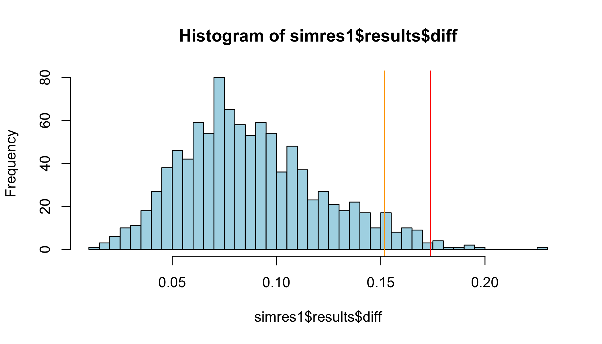
  ..- attr(*, "names")= chr "99%"

The object contains a dataframe with mean and max values for residual correlations within each dataset simulated, and the difference between the mean and the max. This difference is the key metric we are interested in.

The max value will increase with the number of iterations, and it seems to be a bit spurious, so I would suggest to use the 99% percentile value as the cutoff. Based on the simulations I have made so far, it seems that 1000 iterations may be sufficient for a reasonably accurate 99% percentile value (p99) value. For more detailed information on the topic I refer to Christensen et al. (2017).

Code

RIresidcorr(pcmdat2, cutoff = simres1$p99)

	I1	I2	I3
I1
I2	-0.13
I3	-0.29	-0.33
I4	-0.38	-0.44	0.2
Note:
Relative cut-off value (highlighted in red) is -0.052, which is 0.174 above the average correlation (-0.226).

We can see that items 3 and 4 have a residual correlation between them that is quite a bit above the threshold value.

Since the results of the simulation is included in the output object, we can investigate it further.

Code

hist(simres1$results$diff, breaks = 50, col = "lightblue")
abline(v = simres1$p99, col = "red")
abline(v = simres1$p95, col = "orange")

Code

summary(simres1$results$diff)

   Min. 1st Qu.  Median    Mean 3rd Qu.    Max. 
0.01344 0.06429 0.08356 0.08805 0.10804 0.22923

4 Conditional item fit

While conditional item fit is a huge step towards getting correct item fit values (Buchardt et al., 2023; Christensen & Kreiner, 2012; Müller, 2020), we also need to know the range of values that are plausible for items fitting the Rasch model in the current context. The specific properties of the sample and the items is used to simulate multiple datasets that fit the Rasch model, to understand the variation in item fit that can be expected. The simulation results can then be compared with the observed data.

Note

We will use 1000 simulations, but no extensive tests have been made (yet) to determine a reasonable number of simulations. The more items/thresholds and the bigger your sample size, the more time this simulation will take. If you have more cpu cores, this will reduce the time (please remember to not use all cores, leave 1-2 unused).

To give some reference, the code below (n = 300, 4 items, 4 response categories per item) using 500 iterations took 3.7 seconds on 4 cpu cores. 1000 iterations on 8 cores took 4.2 seconds (based on single runs). I recommend library(tictoc) to make timing easy.

Code

simfit1 <- RIgetfit(pcmdat2, iterations = 1000, cpu = 8)

The output is a list object consisting of one dataframe per iteration. We can look at iteration 1:

Code

simfit1[[1]]

  Item InfitMSQ OutfitMSQ
1   I1    0.962     0.969
2   I2    0.964     0.946
3   I3    1.041     1.027
4   I4    1.020     1.023

This object can in turn be used with three different functions. Most importantly, you can use it with RIitemfit() to automatically set the simulation based cutoff values for infit & outfit MSQ based on your sample size and item parameters. RIitemfit() uses the .05 and 99.5 percentile values for each individual item. The cutoff limit might be added as a user option later. You can optionally sort the table output according to misfit by using sort = "infit".

Code

RIitemfit(pcmdat2, simfit1)

Item	InfitMSQ	Infit thresholds	OutfitMSQ	Outfit thresholds	Infit diff	Outfit diff
I1	1.08	[0.853, 1.138]	1.069	[0.835, 1.201]	no misfit	no misfit
I2	1.155	[0.838, 1.169]	1.084	[0.794, 1.256]	no misfit	no misfit
I3	0.828	[0.849, 1.174]	0.802	[0.792, 1.238]	0.021	no misfit
I4	1.007	[0.838, 1.171]	1.024	[0.808, 1.22]	no misfit	no misfit
Note:
MSQ values based on conditional calculations (n = 300). Simulation based thresholds based on 1000 simulated datasets.

The function RIgetfitPlot() uses the package ggdist to plot the distribution of fit values from the simulation results. You can get the observed conditional item fit included in the plot by using the option data = yourdataframe.

Code

RIgetfitPlot(simfit1, pcmdat2)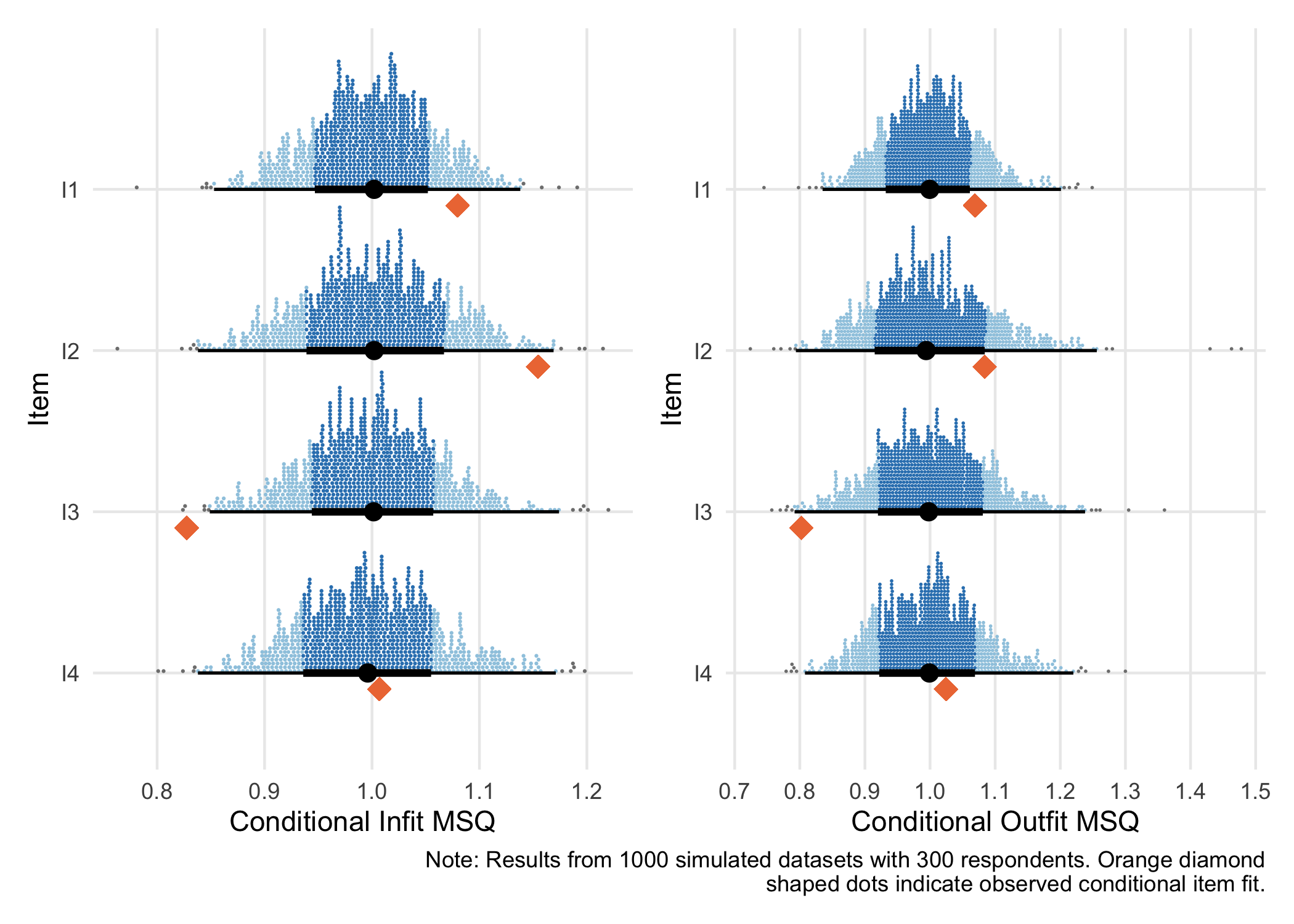

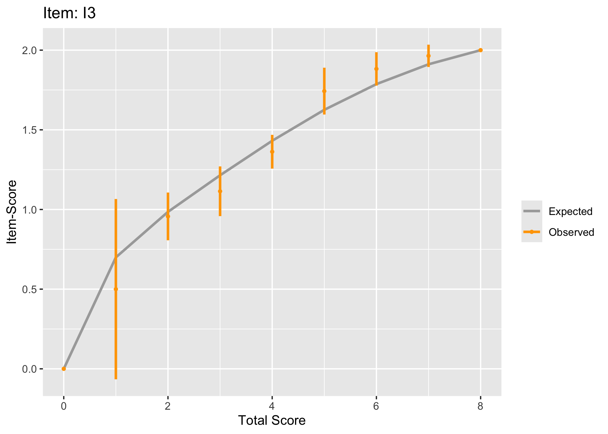
5 Visualizing conditional fit

As a side note, a graphical representation of conditional item fit across class intervals (Buchardt et al., 2023) can be helpful to further analyze our observed data.

Code

library(RASCHplot) # devtools::install_github("ERRTG/RASCHplot")
CICCplot(PCM(pcmdat2), which.item = 3)

$I3

6 Session info

Code

sessionInfo()

R version 4.4.1 (2024-06-14)
Platform: aarch64-apple-darwin20
Running under: macOS Sonoma 14.6.1

Matrix products: default
BLAS:   /Library/Frameworks/R.framework/Versions/4.4-arm64/Resources/lib/libRblas.0.dylib 
LAPACK: /Library/Frameworks/R.framework/Versions/4.4-arm64/Resources/lib/libRlapack.dylib;  LAPACK version 3.12.0

locale:
[1] en_US.UTF-8/en_US.UTF-8/en_US.UTF-8/C/en_US.UTF-8/en_US.UTF-8

time zone: Europe/Stockholm
tzcode source: internal

attached base packages:
 [1] parallel  grid      stats4    stats     graphics  grDevices utils    
 [8] datasets  methods   base     

other attached packages:
 [1] RASCHplot_0.1.0    ggdist_3.3.2       doParallel_1.0.17  iterators_1.0.14  
 [5] foreach_1.5.2      RISEkbmRasch_0.2.4 janitor_2.2.0      iarm_0.4.3        
 [9] hexbin_1.28.3      catR_3.17          glue_1.7.0         ggrepel_0.9.5     
[13] patchwork_1.2.0    reshape_0.8.9      matrixStats_1.3.0  psychotree_0.16-1 
[17] psychotools_0.7-4  partykit_1.2-21    mvtnorm_1.2-5      libcoin_1.0-10    
[21] psych_2.4.6.26     mirt_1.42          lattice_0.22-6     eRm_1.0-6         
[25] lubridate_1.9.3    forcats_1.0.0      stringr_1.5.1      dplyr_1.1.4       
[29] purrr_1.0.2        readr_2.1.5        tidyr_1.3.1        tibble_3.2.1      
[33] ggplot2_3.5.1      tidyverse_2.0.0    kableExtra_1.4.0   formattable_0.2.1 

loaded via a namespace (and not attached):
  [1] later_1.3.2          splines_4.4.1        R.oo_1.26.0         
  [4] cellranger_1.1.0     rpart_4.1.23         lifecycle_1.0.4     
  [7] rstatix_0.7.2        rprojroot_2.0.4      globals_0.16.3      
 [10] MASS_7.3-61          backports_1.5.0      magrittr_2.0.3      
 [13] vcd_1.4-12           Hmisc_5.1-3          rmarkdown_2.27      
 [16] yaml_2.3.10          httpuv_1.6.15        sessioninfo_1.2.2   
 [19] pbapply_1.7-2        RColorBrewer_1.1-3   abind_1.4-5         
 [22] audio_0.1-11         quadprog_1.5-8       R.utils_2.12.3      
 [25] nnet_7.3-19          listenv_0.9.1        testthat_3.2.1.1    
 [28] RPushbullet_0.3.4    vegan_2.6-6.1        parallelly_1.38.0   
 [31] svglite_2.1.3        permute_0.9-7        codetools_0.2-20    
 [34] DT_0.33              xml2_1.3.6           tidyselect_1.2.1    
 [37] farver_2.1.2         base64enc_0.1-3      jsonlite_1.8.8      
 [40] progressr_0.14.0     Formula_1.2-5        survival_3.7-0      
 [43] systemfonts_1.1.0    tools_4.4.1          gnm_1.1-5           
 [46] Rcpp_1.0.13          mnormt_2.1.1         gridExtra_2.3       
 [49] xfun_0.46            here_1.0.1           mgcv_1.9-1          
 [52] distributional_0.4.0 ca_0.71.1            withr_3.0.1         
 [55] beepr_2.0            fastmap_1.2.0        fansi_1.0.6         
 [58] digest_0.6.36        mime_0.12            timechange_0.3.0    
 [61] R6_2.5.1             colorspace_2.1-1     R.methodsS3_1.8.2   
 [64] inum_1.0-5           utf8_1.2.4           generics_0.1.3      
 [67] data.table_1.15.4    SimDesign_2.16       htmlwidgets_1.6.4   
 [70] pkgconfig_2.0.3      gtable_0.3.5         lmtest_0.9-40       
 [73] brio_1.1.5           htmltools_0.5.8.1    carData_3.0-5       
 [76] scales_1.3.0         corrplot_0.92        snakecase_0.11.1    
 [79] knitr_1.48           rstudioapi_0.16.0    reshape2_1.4.4      
 [82] tzdb_0.4.0           checkmate_2.3.2      nlme_3.1-165        
 [85] curl_5.2.1           zoo_1.8-12           cachem_1.1.0        
 [88] relimp_1.0-5         vcdExtra_0.8-5       foreign_0.8-87      
 [91] pillar_1.9.0         vctrs_0.6.5          promises_1.3.0      
 [94] ggpubr_0.6.0         car_3.1-2            xtable_1.8-4        
 [97] Deriv_4.1.3          cluster_2.1.6        dcurver_0.9.2       
[100] GPArotation_2024.3-1 htmlTable_2.4.3      evaluate_0.24.0     
[103] cli_3.6.3            compiler_4.4.1       rlang_1.1.4         
[106] future.apply_1.11.2  ggsignif_0.6.4       labeling_0.4.3      
[109] plyr_1.8.9           stringi_1.8.4        viridisLite_0.4.2   
[112] munsell_0.5.1        Matrix_1.7-0         qvcalc_1.0.3        
[115] hms_1.1.3            future_1.34.0        shiny_1.9.1         
[118] broom_1.0.6          memoise_2.0.1        ggstance_0.3.7      
[121] readxl_1.4.3

7 References

Buchardt, A.-S., Christensen, K. B., & Jensen, N. (2023). Visualizing Rasch item fit using conditional item characteristic curves in R. Psychological Test and Assessment Modeling, 65(2), 206–219.

Christensen, K. B., & Kreiner, S. (2012). Item Fit Statistics. In Rasch Models in Health (pp. 83–104). John Wiley & Sons, Ltd. https://doi.org/10.1002/9781118574454.ch5

Christensen, K. B., Makransky, G., & Horton, M. (2017). Critical Values for Yen’s Q3: Identification of Local Dependence in the Rasch Model Using Residual Correlations. Applied Psychological Measurement, 41(3), 178–194. https://doi.org/10.1177/0146621616677520

Müller, M. (2020). Item fit statistics for Rasch analysis: Can we trust them? Journal of Statistical Distributions and Applications, 7(1), 5. https://doi.org/10.1186/s40488-020-00108-7

Reuse

CC BY 4.0

Citation

BibTeX citation:

@online{johansson2024,
  author = {Johansson, Magnus},
  title = {Simulation Based Cutoff Values for {Rasch} Item Fit and
    Residual Correlations},
  date = {2024-09-27},
  url = {https://pgmj.github.io/simcutoffs.html},
  langid = {en}
}

For attribution, please cite this work as:

Johansson, M. (2024, September 27). Simulation based cutoff values for Rasch item fit and residual correlations. https://pgmj.github.io/simcutoffs.html