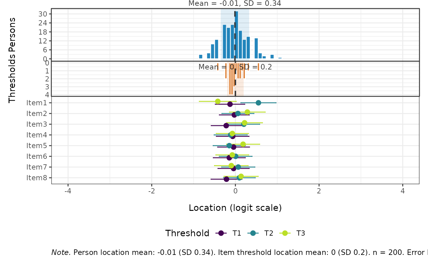
Person-Item Targeting Plot (Wright Map)

Produces a three-panel targeting plot with a shared logit scale x-axis:

Top: Histogram of person location estimates, with a reference line for the mean (or median) and shading for ±1 SD (or ±1 MAD).
Middle: Inverted histogram of item threshold locations, with the same summary annotations.
Bottom: Dot-and-whisker plot of individual item thresholds with confidence intervals based on threshold standard errors.

Usage

RMtargeting(
  data,
  robust = FALSE,
  sort_items = c("data", "location"),
  bins,
  xlim = c(-4, 4),
  ci_level = 0.95,
  person_fill = "#0072B2",
  threshold_fill = "#D55E00",
  height_ratios = c(3, 2, 5),
  output = "figure"
)

Arguments

data: A data.frame or matrix of item responses. Items must be scored starting at 0 (non-negative integers). Missing values (NA) are allowed.
robust: Logical. If FALSE (the default), histogram annotations use mean ± SD. If TRUE, median ± MAD is used instead.
sort_items: Character string controlling item ordering on the y-axis of the bottom panel. "data" (the default) preserves the column order in data (first item at top). "location" sorts items by their average threshold location (easiest at top, hardest at bottom).
bins: Integer. Number of bins for both histograms. Default is number of unique scores plus one, but no less than 15.
xlim: Numeric vector of length 2. Initial lower and upper limits for the shared x-axis. Automatically expanded if any person or item threshold values fall outside these limits.
ci_level: Numeric. Confidence level for the item threshold error bars. Default is 0.95 (95% CI). Set to NULL to hide error bars.
person_fill: Fill colour for the person histogram. Default "#0072B2" (blue).
threshold_fill: Fill colour for the item threshold histogram. Default "#D55E00" (vermillion).
height_ratios: Numeric vector of length 3 specifying the relative heights of the top (person), middle (threshold), and bottom (dot-whisker) panels. Default c(3, 2, 5).
output: Character string. "figure" (the default) returns the combined patchwork plot. "list" returns a named list of the three ggplot objects (p1, p2, p3) for further customisation.

Value

If output = "figure": a patchwork object (combined ggplot).
If output = "list": a named list with elements p1 (person histogram), p2 (threshold histogram), and p3 (item threshold dot-whisker plot).

Details

Together, the top and middle panels form a back-to-back histogram that makes it easy to assess whether the test is well-targeted to the sample.

Estimation method selection. The function checks whether any item response category has fewer than 3 observations. If all categories have at least 3 responses, item threshold locations and their standard errors are estimated via Conditional Maximum Likelihood (CML) using eRm::RM() (dichotomous) or eRm::PCM() (polytomous), with SEs from eRm::thresholds(). If any category has fewer than 3 responses, the function falls back to Marginal Maximum Likelihood (MML) estimation via mirt::mirt() with itemtype = "Rasch" and SE = TRUE, which is more numerically stable under sparse-category conditions. A message is emitted when the MML fallback is used.

In both cases, item threshold locations are centered (shifted so the grand mean of all thresholds equals zero).

Person estimates are obtained via Maximum Likelihood (ML) from eRm::person.parameter(), which uses spline interpolation to extrapolate location estimates for persons with extreme scores (all-zero or perfect). Persons for whom the spline interpolation fails receive NA and are excluded from the histogram.

Confidence intervals for item thresholds are based on Wald-type intervals: threshold estimate ± z × SE, where z is the standard normal quantile corresponding to ci_level.

The ggplot2 and patchwork packages must be installed (they are in Suggests, not Imports).

References

Wright, B. D. & Stone, M. H. (1979). Best Test Design. MESA Press.

Examples

# \donttest{
# Polytomous example
set.seed(42)
sim_data <- as.data.frame(
  matrix(sample(0:3, 200 * 8, replace = TRUE), nrow = 200, ncol = 8)
)
colnames(sim_data) <- paste0("Item", 1:8)

# Default: mean/SD, data order, 95% CI
RMtargeting(sim_data)


# Robust (median/MAD), sorted by location, 84% CI
RMtargeting(sim_data, robust = TRUE, sort_items = "location", ci_level = 0.84)


# Get list of sub-plots for customisation
plots <- RMtargeting(sim_data, output = "list")
plots$p1 + ggplot2::ggtitle("My custom title")


# Dichotomous example
sim_bin <- as.data.frame(
  matrix(sample(0:1, 200 * 10, replace = TRUE), nrow = 200, ncol = 10)
)
colnames(sim_bin) <- paste0("Item", 1:10)
RMtargeting(sim_bin)

# }