Plot the Simulated Item-Restscore Null Distribution
Source:R/item_restscore_plot.R
RMitemRestscorePlot.RdVisualises the per-item null distribution of the observed minus expected
item-restscore gamma from RMitemRestscoreCutoff, optionally
overlaying the observed differences from the original data.
Arguments
- simfit
The return value of
RMitemRestscoreCutoff(a list with componentsresults,item_cutoffs,actual_iterations,sample_n, anditem_names).- data
Optional. A data.frame or matrix of item responses for computing and overlaying the observed item-restscore differences. Items must be scored starting at 0 (non-negative integers). When provided, the plot includes orange diamond markers for the observed difference alongside the simulated distribution, plus segment summaries of the intervals.
Details
Uses ggdist::stat_dotsinterval() (when data is not supplied) or
ggdist::stat_dots() (when data is supplied) with
point_interval = "median_hdci". The outer .width follows
simfit$hdci_width, so the shaded interval matches the one
RMitemRestscore() tabulates.
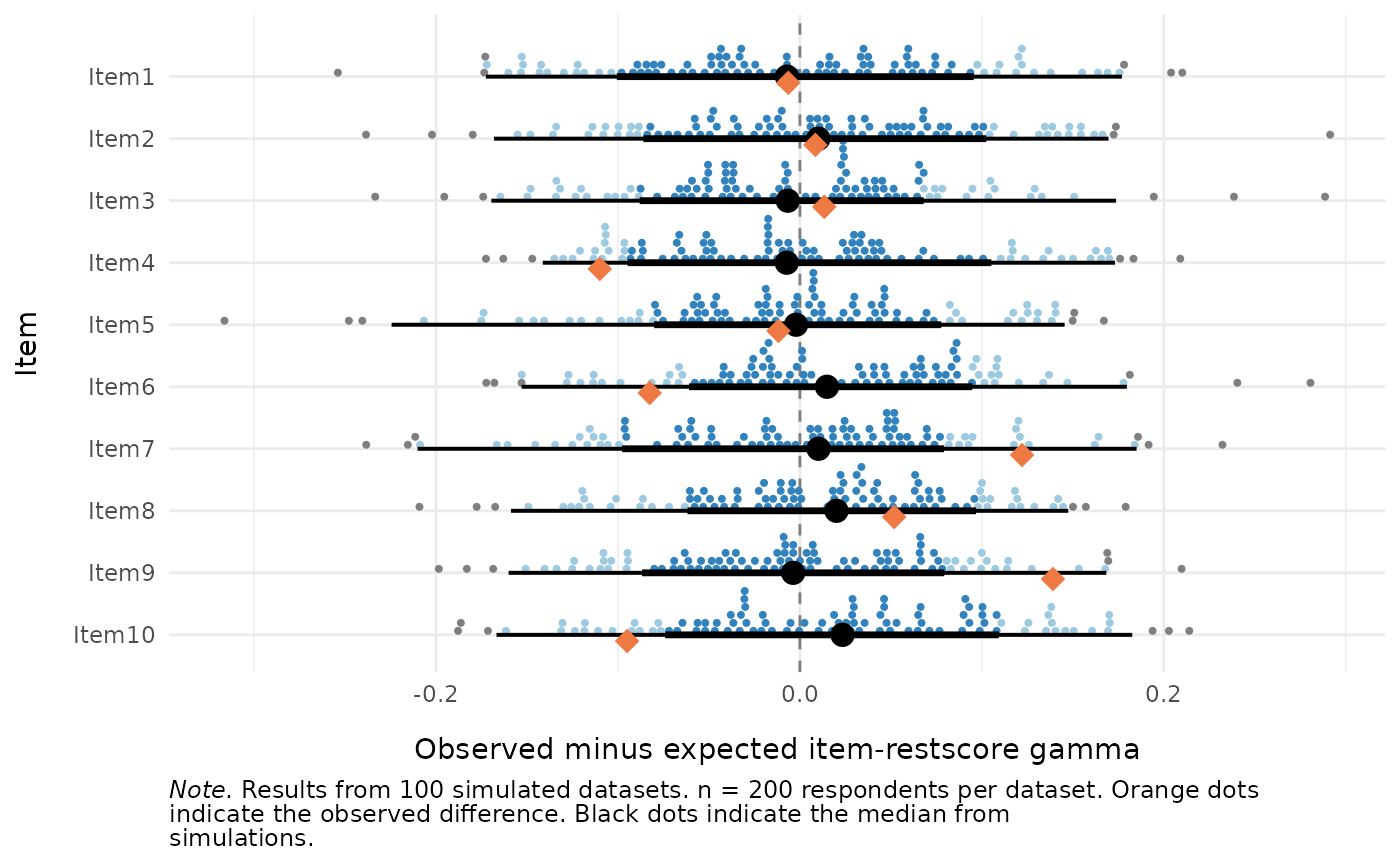
The x-axis is the difference between observed and model-expected gamma, the
statistic RMitemRestscore tests. A dashed line marks zero.
The simulated distributions are generally not centred on zero in small
samples, which is one of the reasons the asymptotic test is miscalibrated
(see RMitemRestscoreCutoff). Positive values indicate
over-discrimination (overfit), negative values under-discrimination
(underfit).
When data is supplied, the observed differences are computed with
RMitemRestscore and overlaid as orange diamonds, with per-item
intervals drawn as black line segments (thicker for the 66% range) and
black dots for the simulated median.
The ggplot2 and ggdist packages must be installed (they are in
Suggests, not Imports).
Examples
# \donttest{
if (requireNamespace("iarm", quietly = TRUE) &&
requireNamespace("ggdist", quietly = TRUE) &&
requireNamespace("ggplot2", quietly = TRUE)) {
set.seed(42)
sim_data <- as.data.frame(
matrix(sample(0:1, 200 * 10, replace = TRUE), nrow = 200, ncol = 10)
)
colnames(sim_data) <- paste0("Item", 1:10)
cutoff_res <- RMitemRestscoreCutoff(sim_data, iterations = 100,
parallel = FALSE, seed = 42)
# Simulated distribution only
RMitemRestscorePlot(cutoff_res)
# With the observed differences overlaid
RMitemRestscorePlot(cutoff_res, data = sim_data)
}
#>
 # }
# }