A brief comparison of test equating methods

library(dplyr)
library(tidyr)
library(ggplot2)
library(leunbachR)
library(equate)
library(SNSequate)
library(knitr)
library(mirt)
library(kequate)

set.seed(1234) # for reproducibility of bootstrap results
select <- dplyr::select

d3a_sum <- read.delim("data/data3a_item.csv", sep = ",") %>% 
  select(a01:a10,b01:b10) %>% 
  mutate(a_sum = rowSums(across(c(a01:a10))),
         b_sum = rowSums(across(c(b01:b10)))) %>% 
  select(a_sum,b_sum)

d3a <- read.delim("data/data3a_item.csv", sep = ",") %>% 
  select(a01:a10,b01:b10)

head(d3a)

##   a01 a02 a03 a04 a05 a06 a07 a08 a09 a10 b01 b02 b03 b04 b05 b06 b07 b08 b09
## 1   0   0   0   1   0   0   0   0   0   0   1   1   0   0   0   0   1   0   0
## 2   1   1   0   0   1   0   0   1   0   0   1   1   1   1   0   0   0   0   0
## 3   1   0   1   0   1   1   0   0   0   0   1   1   1   1   1   1   1   1   1
## 4   1   1   1   1   1   0   1   0   0   0   1   1   1   1   1   1   0   0   0
## 5   1   1   1   1   1   1   1   1   0   0   1   1   1   0   1   0   1   1   0
## 6   1   1   1   0   1   1   1   0   0   0   1   1   1   1   1   0   0   1   1
##   b10
## 1   0
## 2   0
## 3   0
## 4   0
## 5   0
## 6   1

While the Leunbach method allows for test equating based on observed sum scores under the assumption that the underlying data fits a Rasch model adequately, most other methods require item-level response data.

We will first focus on comparing IRT true score equating to Leunbach, but also include some other methods.

Direct equating

mod1 <- mirt(d3a[,1:10], 1, 'Rasch', verbose = FALSE) 
mod2 <- mirt(d3a[,11:20], 1, 'Rasch', verbose = FALSE) 

coef_ls1 <- list(a = rep(1,10), 
                 b = coef(mod1, simplify=TRUE, IRTpars = TRUE)$item[,'b'],
                 c = rep(0,10))
coef_ls2 <- list(a = rep(1,10), 
                 b = coef(mod2, simplify=TRUE, IRTpars = TRUE)$item[,'b'],
                 c = rep(0,10))

req1 <- irt.eq(n_items = 10, coef_ls1, coef_ls2, method="TS", A=1, B=0) # true score
rx <- freqtab(rowSums(d3a[,1:10]), scales = 0:10) 
ry <- freqtab(rowSums(d3a[,11:20]), scales = 0:10) 
req2 <- equate(rx, ry, type = "i") # identity 
req3 <- equate(rx, ry, type = "l") # linear 
req4 <- equate(rx, ry, type = "e", smooth = "loglin", degrees = 3) # equipercentile with loglinear smoothing

# Leunbach model
lfit <- leunbach_ipf(d3a_sum)
lboot <- leunbach_bootstrap(lfit, n_cores = 4, nsim = 100)
leq <- get_equating_table(lboot)

# summary table
max_score <- 10 
eq_table <- data.frame(identity = pmin(pmax(req2$conc$yx, 0), max_score), 
                       linear = pmin(pmax(req3$conc$yx, 0), max_score), 
                       equiperc_loglin3 = pmin(pmax(req4$conc$yx, 0), max_score),
                       IRT_truescore = req1$tau_y, 
                       leunbach_expected = leq$expected,
                       IRT_thetaequivalent = req1$theta_equivalent,
                       leunbach_theta = leq$log_theta
                       ) %>% 
  round(2)

kable(eq_table)

identity	linear	equiperc_loglin3	IRT_truescore	leunbach_expected	IRT_thetaequivalent	leunbach_theta
0	0.36	0.00	0.00	0.00	NA	-5.00
1	1.30	0.96	0.91	0.79	-2.18	-1.98
2	2.23	2.10	1.93	1.90	-1.49	-1.33
3	3.16	3.19	2.99	3.07	-0.94	-0.86
4	4.10	4.20	4.04	4.16	-0.45	-0.45
5	5.03	5.14	5.08	5.11	0.02	-0.07
6	5.97	6.03	6.10	5.95	0.49	0.29
7	6.90	6.88	7.09	6.71	0.98	0.66
8	7.84	7.64	8.08	7.53	1.51	1.13
9	8.77	8.42	9.06	8.80	2.19	2.01
10	9.71	9.38	10.00	10.00	NA	5.00

eq_table %>% 
  select(!c(leunbach_theta,IRT_thetaequivalent)) %>% 
  pivot_longer(!identity) %>% 
  ggplot(aes(x = identity, y = value, color = name, shape = name, linetype = name)) +
  geom_point(size = 2.5) + 
  geom_line() +
  scale_x_continuous(breaks = c(0:10), minor_breaks = NULL) +
  scale_y_continuous(breaks = c(0:10)) +
  scale_color_viridis_d() +
  theme_bw() +
  labs(title = "Test equating on sum score scale",
       color = "Equating model", shape = "Equating model", linetype = "Equating model",
       y = "Predicted Y value", x = "X value")

eq_table %>% 
  select(c(identity,leunbach_theta,IRT_thetaequivalent)) %>% 
  pivot_longer(!identity) %>% 
  filter(identity %in% c(1:9)) %>% 
  ggplot(aes(x = identity, y = value, color = name, shape = name)) +
  geom_point(size = 3) + 
  geom_line() +
  scale_x_continuous(breaks = c(0:10), minor_breaks = NULL) +
  scale_y_continuous(breaks = c(-2:2)) +
  scale_color_viridis_d() +
  theme_bw() +
  labs(title = "Test equating on theta scale",
       color = "Equating model", shape = "Equating model",
       y = "Predicted Y value", x = "X value", caption = "Note: Min and max scores are excluded, since these need to be imputed for both methods.") +
  theme(plot.caption = element_text(face = "italic", hjust = 0))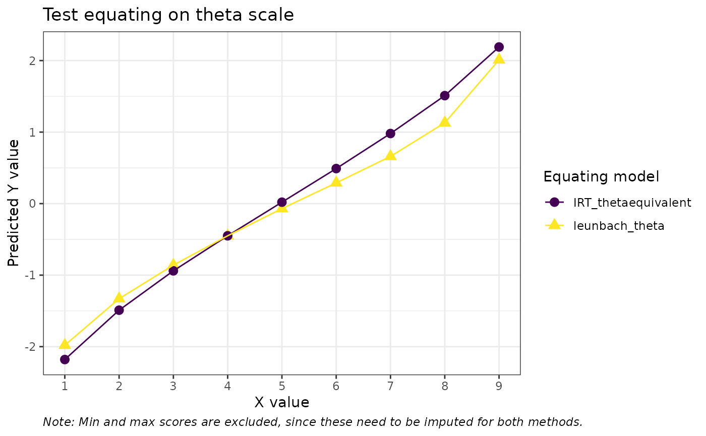

Kernel equating

We’ll apply the equivalent groups design, following the kequate package vignette (Andersson, Bränberg, and Wiberg 2022). First, we fit two separate generalized linear models (GLM) using the poisson distribution for the counts of each score. The kequate vignette suggests using AIC to evaluate model fit (lower values are better) and finding the optimal number of moments to include in the model specification. I have opted for using B-splines instead for slightly improved model fit, and adjusting the degrees of freedom based on AIC. The glm() output objects are then used by the kequate() function.

Notably, like Leunbach, kernel equating also allows for equating using only sum scores.

glm_a <- glm(count ~ splines::bs(total, df = 3),
  family = "poisson", data = rx, x = TRUE)
glm_b <- glm(count ~ splines::bs(total, df = 3),
  family = "poisson", data = ry, x = TRUE)

Bias correction following Kosmidis et al. (2020).

library(brglm2)
glm_a2 <- update(glm_a, method = "brglmFit")
glm_b2 <- update(glm_b, method = "brglmFit")
eg_eq <- kequate(
  design = "EG",
  r = glm_a2, s = glm_b2,
  x = c(0:10), y = c(0:10)
)

data.frame(
  predicted = c(eg_eq@equating$eqYx, leq$expected),
  Model = c(rep("Kernel equating",11),rep("Leunbach",11)),
  sumscore = c(0:10,0:10)
  ) %>% 
  ggplot(aes(x = sumscore, y = predicted, color = Model, shape = Model)) +
  geom_point(size = 3) + 
  geom_line() +
  scale_x_continuous(breaks = c(0:10), minor_breaks = NULL) +
  #scale_y_continuous(breaks = c(-2:2)) +
  scale_color_viridis_d() +
  theme_bw() +
  labs(title = "Test equating expected scores",
       color = "Equating model", shape = "Equating model",
       y = "Predicted Y value", x = "X value") +
  theme(plot.caption = element_text(face = "italic", hjust = 0))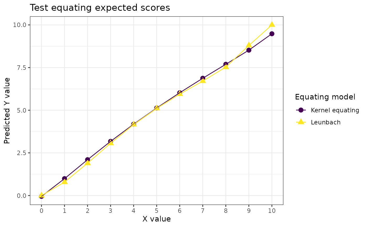

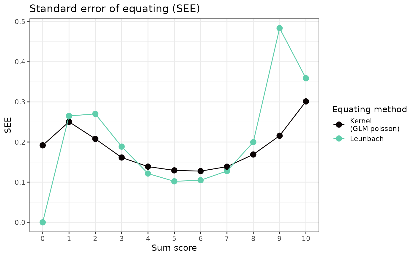
Standard error of equating

In order to make reasonable comparisons between kernel equating and Leunbach, we need to use the expected values for estimating standard errors of equating (SEE) in the Leunbach bootstrap, rather than the rounded values (default). It should be noted that the methods of estimating SEE are different for these two equating models.

lboot2 <- leunbach_bootstrap(lfit, n_cores = 4, nsim = 100, see_type = "expected")

data.frame(score = c(0:10,0:10),
           see = c(lboot2[["see_1to2"]],eg_eq@equating$SEEYx),
           model = c(rep("Leunbach",11),rep("Kernel\n(GLM poisson)",11))
) %>% ggplot(aes(x=score,y=see, color = model)) +
  geom_point(size = 3) +
  geom_line() +
  theme_bw() +
  scale_x_continuous(breaks = c(0:10), minor_breaks = NULL) +
  scale_color_viridis_d(option = "G", end = 0.8) +
  labs(title = "Standard error of equating (SEE)",
       x = "Sum score", y = "SEE", color = "Equating method")

References

Andersson, Björn, Kenny Bränberg, and Marie Wiberg. 2022. “Kequate: The Kernel Method of Test Equating.” https://cran.uni-muenster.de/web/packages/kequate/index.html.

Kosmidis, Ioannis, Euloge Clovis Kenne Pagui, and Nicola Sartori. 2020. “Mean and Median Bias Reduction in Generalized Linear Models.” Statistics and Computing 30 (1): 43–59. https://doi.org/10.1007/s11222-019-09860-6.

Magnus Johansson, PhD

2026-02-04

Direct equating

Kernel equating

Standard error of equating

References