Conditional measurement precision across the latent scale

Plots (or tabulates) how precisely a scale measures at each point of the latent continuum, rather than collapsing precision to the single number reported by RMreliability(). The curve is the conditional standard error of measurement $SEM(\theta) = 1/\sqrt{I(\theta)}$, the test information $I(\theta)$ it comes from, or the conditional reliability derived from either.

Usage

RMreliabilityCurve(
  data,
  statistic = "sem",
  method = "WLE",
  benchmark = NULL,
  reference = "marginal",
  items = NULL,
  item_params = NULL,
  boot = FALSE,
  boot_iter = 200,
  conf_int = 0.95,
  parallel = TRUE,
  n_cores = NULL,
  seed = NULL,
  show_density = TRUE,
  theta_range = NULL,
  n_nodes = 161L,
  verbose = FALSE,
  output = "ggplot"
)

Arguments

data: A data.frame or matrix of item responses. Items must be scored starting at 0 (non-negative integers). Missing values (NA) are allowed.
statistic: Character. The quantity on the y-axis: "sem" (default, the conditional standard error in logits), "information" (test information), or "reliability" (see Details for the formula used, and why). This is the argument that chooses what the figure shows, not method.
method: Character. Person-location estimator, "WLE" (default) or "EAP". This does not change the curve, which is always built from test information. It governs only the respondent locations behind the density overlay and the benchmark percentage, and is ignored when show_density = FALSE and benchmark = NULL.
benchmark: Numeric in (0, 1) or NULL (default). When supplied, the region of the scale whose conditional reliability reaches benchmark is shaded, and the percentage of respondents located inside it is reported. There is deliberately no default value; see Details.
reference: Character. Horizontal line showing the flat summary that a single coefficient implies: "marginal" (default) or "none".
items: Optional character vector of column names, or numeric column indices, selecting a subset of items. Useful for comparing a short form against the full scale.
item_params: Optional pre-specified item parameters, used in place of the thresholds estimated from data. Either a named list of Andrich threshold vectors or a long-format data.frame from RMitemParameters(), the same two forms RMpersonParameters() accepts. Supply this to draw the curve from anchored or previously published parameters. As in RMpersonParameters(), supplied thresholds are used as given and are not re-centred, so their origin defines the origin of the theta axis.
boot: Logical. If TRUE, add a bootstrap confidence band to the curve by resampling respondents. Default FALSE.
boot_iter: Integer. Bootstrap iterations when boot = TRUE. Default 200.
conf_int: Numeric in (0, 1). HDCI width for the bootstrap band. Default 0.95.
parallel: Logical. Use mirai for the bootstrap if available. Default TRUE.
n_cores: Integer or NULL. Number of parallel workers. When NULL, getOption("mc.cores") is checked first; if neither is set, the bootstrap falls back to sequential.
seed: Integer or NULL. Random seed for the bootstrap. See easyRasch2-reproducibility.
show_density: Logical. Draw the respondent location distribution as a background band. Default TRUE.
theta_range: Numeric length-2 vector, or NULL (default) for $\pm 3\sigma$.
n_nodes: Integer. Number of points on the theta grid. Default 161.
verbose: Logical. Print a progress bar for the bootstrap. Default FALSE.
output: Character. "ggplot" (default), "dataframe" for the curve, or "kable" for a summary table.

Value

If output = "ggplot": a ggplot object.
If output = "dataframe": a data.frame with one row per grid point and columns theta, information, sem, reliability, plus <statistic>_lower / <statistic>_upper band columns when boot = TRUE. Attributes carry the summary quantities: sigma, marginal_ratio (the latent-density-weighted mean of the reliability curve, matching RMreliability()), marginal_green (the superseded subtractive coefficient), sem_average (root mean error variance), latent_mean, benchmark, benchmark_range, benchmark_percent and n_not_estimable.

latent_mean and sigma are estimated together. Before 1.3.1 the mean was held at 0 and $\sigma$ absorbed any distance between the sample and the item locations: on simulated data with a true SD of 0.90, shifting the sample 2 logits off target returned 2.02 rather than 0.96, and pushed marginal reliability from 0.81 up to 0.90 when it should have fallen to 0.73. Well-targeted samples are unaffected.
If output = "kable": a knitr_kable summary table of those quantities.

Details

What the curve is. Test information $I(\theta) = \sum_i \mathrm{Var}_i(\mathrm{score} \mid \theta)$ is summed from the CML item thresholds (psychotools), and the conditional standard error follows as $1/\sqrt{I(\theta)}$. Both are properties of the item set alone. The respondent distribution is drawn behind the curve because precision only matters where people actually are, but it does not enter the curve.

Conditional reliability, and which formula. Two definitions circulate:

$$\rho(\theta) = \frac{\sigma^2}{\sigma^2 + SEM(\theta)^2} \qquad \mathrm{and} \qquad \rho(\theta) = 1 - \frac{SEM(\theta)^2}{\sigma^2}$$

with $\sigma$ the latent SD estimated by marginal maximum likelihood, jointly with the latent mean $\mu$ (see the latent_mean attribute). This function uses the first, the ratio form, for three reasons. It is bounded in (0, 1), whereas the subtractive form returns negative values whenever $SEM(\theta) > \sigma$, which is common at the floor of a skewed scale and at both tails of a short one. It treats $\sigma^2$ as true-score variance, which is what the MML estimate of the latent SD is. And it tracks the reliability of the observed scores far more closely. Milanzi et al. (2015) report the subtractive coefficient falling to $-0.120$ against a true value of $0.480$ for a 1PL with $\sigma^2 = 0.25$. Replicating their design (dev/milanzi_check.R, 1000 replications per cell) gives a mean absolute error against the exact expected-sum-score reliability of $0.22$ for the subtractive form and $0.018$ for the ratio form, with the subtractive form negative in 99.7% of replications of their lowest-variance cell. For polytomous Rasch data at 5 to 20 items the corresponding errors are $0.18$ and $0.015$.

The advantage is concentrated where it matters rather than uniform. Where information is high relative to the trait variance the two forms are close and either can be nearer the truth. The gap comes from the low-information cases, where the subtractive form does not merely lose accuracy but leaves the (0, 1) interval altogether.

marginal_ratio is the latent-density-weighted mean of the reliability curve rather than the ratio formed from the averaged error variance. The two differ by Jensen's inequality, and the curve mean is the more accurate of the pair (mean absolute error 0.015 against 0.018 for binary data, 0.010 against 0.015 for polytomous).

RMreliability() reports the same ratio-form coefficient in its "Marginal (curve mean)" row, so the scalar and the curve agree. The superseded subtractive value is still returned as marginal_green for comparison with easyRasch2 1.2.0 and earlier, and with mirt::marginal_rxx() and similar software.

Limits. The information-based standard error is asymptotic, and is only an approximation for short scales; Milanzi et al. (2015) find the worst behaviour with six items. The curve describes the precision of the person location estimate on the logit scale, which is not the same quantity as the reliability of a raw sum score, and reliability computed on a latent scale is consistently higher than its manifest counterpart. Use RMscoreSE() for the raw-score view.

No default benchmark. benchmark is NULL unless asked for, in keeping with the package's treatment of fixed rules of thumb. McNeish and Dumas (2025), whose respondent-weighted summary this borrows, are explicit that their own interpretive percentages are heuristic and should not be used as cutoffs.

References

Green, B. F., Bock, R. D., Humphreys, L. G., Linn, R. L., & Reckase, M. D. (1984). Technical Guidelines for Assessing Computerized Adaptive Tests. Journal of Educational Measurement, 21(4), 347-360. doi:10.1111/j.1745-3984.1984.tb01039.x

McNeish, D., & Dumas, D. (2025). Reliability representativeness: How well does coefficient alpha summarize reliability across the score distribution? Behavior Research Methods, 57(3), 93. doi:10.3758/s13428-025-02611-8

Milanzi, E., Molenberghs, G., Alonso, A., Verbeke, G., & De Boeck, P. (2015). Reliability measures in item response theory: Manifest versus latent correlation functions. British Journal of Mathematical and Statistical Psychology, 68(1), 43-64. doi:10.1111/bmsp.12033

Examples

# \donttest{
if (requireNamespace("ggplot2", quietly = TRUE)) {
  # Conditional SEM across the scale
  RMreliabilityCurve(phq9[, 1:9])

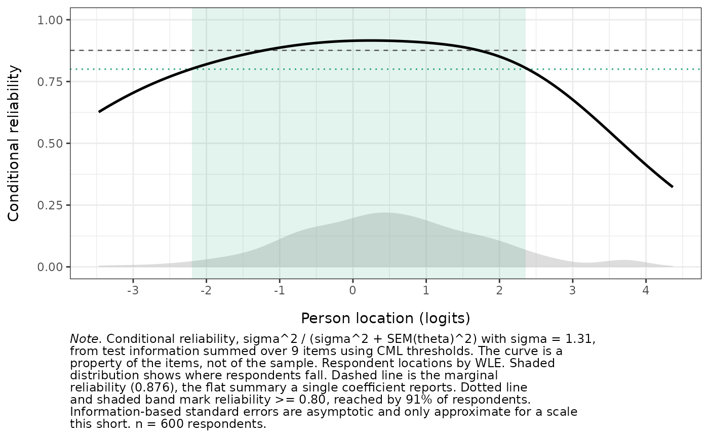
  # Conditional reliability, with the region reaching .8 shaded
  RMreliabilityCurve(phq9[, 1:9], statistic = "reliability",
                     benchmark = 0.8)
}


# Summary quantities
RMreliabilityCurve(phq9[, 1:9], benchmark = 0.8, output = "kable")
#> 
#> 
#> Table: Conditional measurement precision. Test information summed over 9 items from CML thresholds, respondent locations by WLE. Conditional reliability is the ratio form, sigma^2 / (sigma^2 + SEM^2). n = 600 respondents.
#> 
#> |Quantity                                               |Value         |
#> |:------------------------------------------------------|:-------------|
#> |Latent SD (sigma)                                      |1.306         |
#> |Marginal reliability (curve mean, as in RMreliability) |0.876         |
#> |Marginal reliability (Green/Lord, superseded)          |0.845         |
#> |Average SEM (logits)                                   |0.514         |
#> |Minimum SEM (logits)                                   |0.396         |
#> |Theta at minimum SEM                                   |0.25          |
#> |Theta range with reliability >= 0.80                   |-2.20 to 2.36 |
#> |Respondents located in that range                      |91.3%         |
# }