Hurdle Partial Credit Model with easyRaschBayes

Overview

Symptom questionnaires given to a general population sample often have many responses in the lowest category. On the PHQ-9 depression screener, most people answer “Not at all” to most items. A partial credit model (PCM) treats the step from 0 to 1 as one more threshold on the same latent variable as the steps between the higher categories. That may not hold. Not having a symptom at all and how often a present symptom occurs can be different processes.

The hurdle partial credit model (hPCM) separates the two. For each person and item:

• a hurdle submodel, a dichotomous Rasch model, gives the probability of any response above 0 (the symptom is present), and
• a severity submodel, a partial credit model, gives the probability of each category 1, 2, 3 given that the response is above 0.

For person p and item i with categories 0, 1, \dots, m_i, the hurdle submodel is

\operatorname{logit} P(Y_{pi} > 0) = \zeta_p - \delta_i ,

where \zeta_p is the person’s hurdle location and \delta_i the item’s hurdle location. Given a response above 0, the severity submodel is

P(Y_{pi} = k \mid Y_{pi} > 0) = \frac{\exp \sum_{j=2}^{k} (\theta_p - \tau_{ij})} {\sum_{h=1}^{m_i} \exp \sum_{j=2}^{h} (\theta_p - \tau_{ij})}, \qquad k = 1, \dots, m_i ,

where \theta_p is the person’s severity location, \tau_{ij} is the threshold between categories j - 1 and j, and an empty sum is 0. Item i thus has m_i - 1 severity thresholds, two for the PHQ-9 items. The person locations follow a bivariate normal distribution,

\begin{pmatrix} \zeta_p \\ \theta_p \end{pmatrix} \sim \mathcal{N}\left( \begin{pmatrix} 0 \\ 0 \end{pmatrix}, \begin{pmatrix} \sigma_\zeta^2 & \rho \sigma_\zeta \sigma_\theta \\ \rho \sigma_\zeta \sigma_\theta & \sigma_\theta^2 \end{pmatrix} \right).

Each submodel thus has its own person location, and the two are allowed to correlate. The correlation shows whether presence and severity are close to the same trait or two distinct ones. The two correlated traits come from the zero-inflated graded response model of Magnus and Garnier-Villarreal (2022). The hPCM is the Rasch counterpart of the hurdle version of that model (Magnus and Liu 2022), with partial credit in place of graded response. In a hurdle model every zero comes from the hurdle submodel: everyone can have the symptom, and a zero means that it was not reported, not that it could not occur.

The model is fitted with the custom brms (Bürkner 2021) family hurdle_acat(), contributed by Kristoffer Magnusson. The functions with the suffix _hpcm analyse the fitted model.

brms version. On CRAN brms (2.23), custom ordinal families with grouped thresholds produce invalid Stan code. Until a fixed version is on CRAN, install the patched branch to run the code in this vignette:

remotes::install_github("rpsychologist/brms@fix-custom-ordinal-grouped-thres")

The output shown here was computed beforehand with that version. For the standard Rasch workflow, see the partial credit model vignette.

library(easyRaschBayes)
library(brms)
library(dplyr)
library(tidyr)
library(tibble)
library(ggplot2)

Data

phq9_nhanes is a simple random sample of 1000 respondents to the PHQ-9 (Kroenke et al. 2001) in the U.S. National Health and Nutrition Examination Survey (NHANES, September 2024 release), drawn from everyone who answered all nine items. There was no selection on scores, so the share of zero responses is that of a general population sample. See ?phq9_nhanes. Each item is scored 0 (“Not at all”), 1 (“Several days”), 2 (“More than half the days”) and 3 (“Nearly every day”).

data(phq9_nhanes)
items <- phq9_nhanes[, 1:9]

sum_score <- rowSums(items)
summary(sum_score)
#>    Min. 1st Qu.  Median    Mean 3rd Qu.    Max. 
#>   0.000   1.000   3.000   4.416   6.250  24.000
mean(sum_score == 0)  # share with a sum score of zero
#> [1] 0.216
round(colMeans(items == 0), 2)  # share of zero responses per item
#>   q1   q2   q3   q4   q5   q6   q7   q8   q9 
#> 0.63 0.62 0.48 0.40 0.67 0.71 0.70 0.84 0.94

plot_stackedbars(items)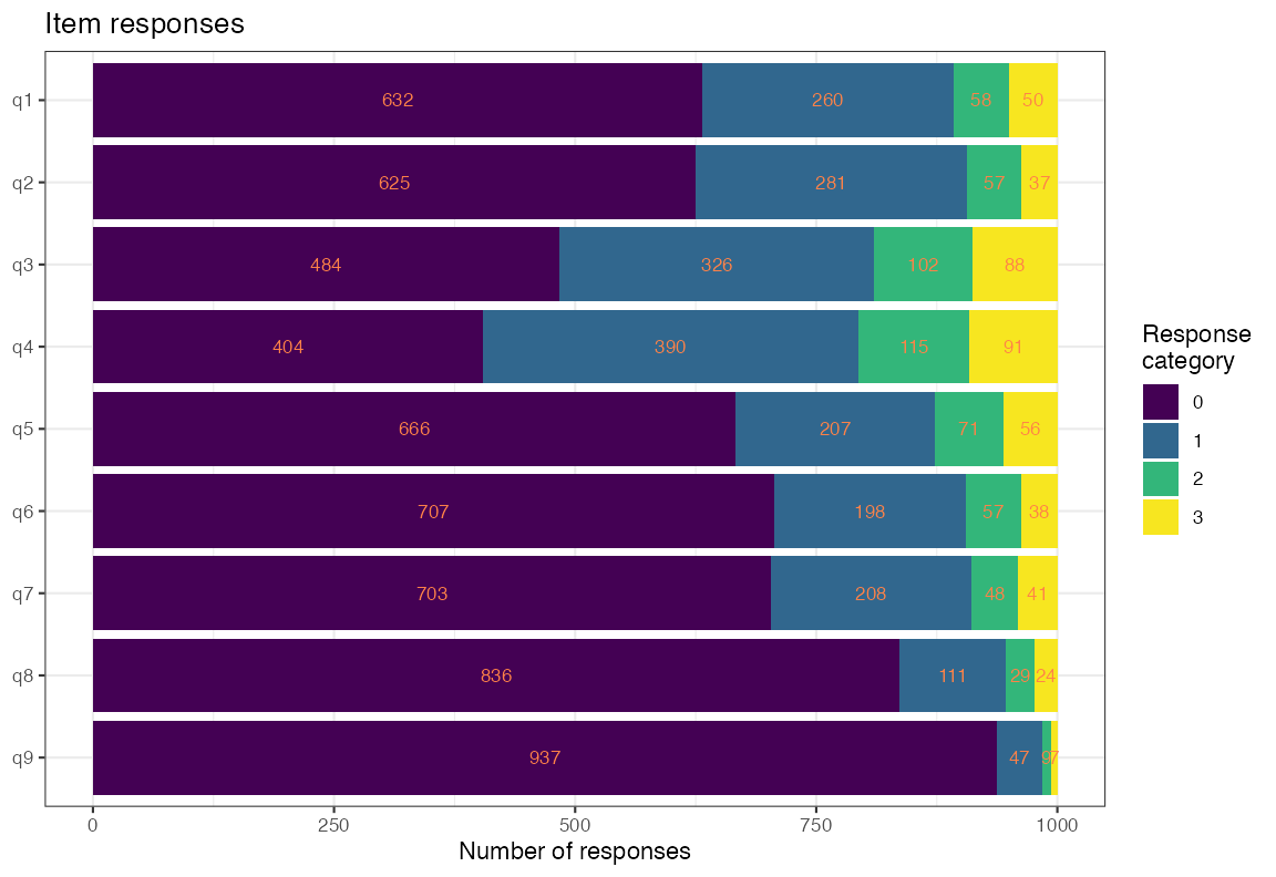

Figure 1. Response distribution per item

The highest categories are rare for several items. On q9 (thoughts of being better off dead or of self-harm), about 1% chose “Nearly every day”. The severity submodel estimates its thresholds from the responses above 0 only, so these thresholds will be uncertain.

For brms, the data go to long format, one row per person and item. The hurdle family uses the responses as they are, coded from 0, since category 0 is the hurdle. The ordinary PCM below needs categories starting at 1, so it gets a separate response column.

df_hpcm <- items %>%
  rownames_to_column("id") %>%
  pivot_longer(!id, names_to = "item", values_to = "response") %>%
  mutate(response_pcm = response + 1)

head(df_hpcm)
#> # A tibble: 6 × 4
#>   id    item  response response_pcm
#>   <chr> <chr>    <int>        <dbl>
#> 1 1     q1           0            1
#> 2 1     q2           0            1
#> 3 1     q3           1            2
#> 4 1     q4           0            1
#> 5 1     q5           0            1
#> 6 1     q6           0            1

A partial credit model first

To see the problem the hurdle model addresses, we first fit an ordinary PCM.

fit_pcm <- brm(
  response_pcm | thres(gr = item) ~ 1 + (1 | id),
  data   = df_hpcm,
  family = acat,
  prior  = prior("normal(0, 3)", class = "Intercept") +
    prior("normal(0, 3)", class = "sd", group = "id"),
  chains = 4, cores = 4, iter = 2000
)
saveRDS(fit_pcm, "fits/fit_pcm_nhanes.rds")

fit_pcm <- readRDS("fits/fit_pcm_nhanes.rds")

plot_targeting(fit_pcm, height_ratios = c(2, 1.5, 7))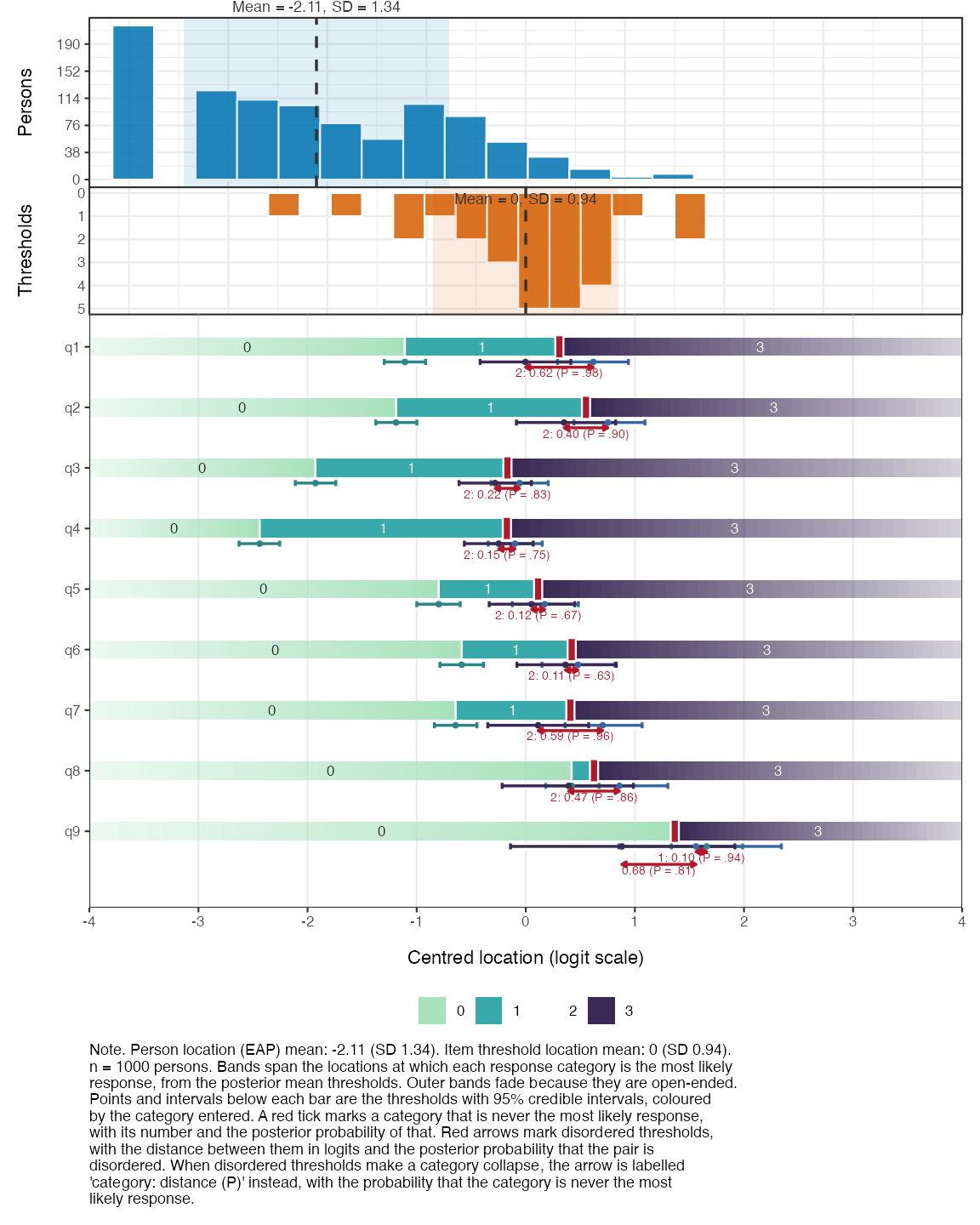

Figure 2. Targeting, partial credit model

The 216 persons with a sum score of zero all get the same, lowest, location and form the spike at the left of the person histogram. The PCM cannot tell them apart. The item panel shows a second problem: for eight of the nine items, category 2 (“More than half the days”) is never the most likely response, because its thresholds are disordered. The PCM places the step from 0 to 1 and the steps between the higher categories on one scale, and in these data they do not line up.

infit_pcm <- infit_post(infit_statistic(fit_pcm, ndraws_use = 500))
infit_pcm$summary
#> # A tibble: 9 × 4
#>   item  infit_obs infit_rep infit_ppp
#>   <chr>     <dbl>     <dbl>     <dbl>
#> 1 q1        1.04      1         0.758
#> 2 q2        0.797     1.01      0.002
#> 3 q3        1.27      0.997     1    
#> 4 q4        1.01      0.999     0.566
#> 5 q5        1.17      1         0.994
#> 6 q6        0.872     1.00      0.046
#> 7 q7        1.04      1.00      0.706
#> 8 q8        1.18      1.00      0.93 
#> 9 q9        0.922     1.00      0.32

rest_pcm <- item_restscore_post(item_restscore_statistic(fit_pcm, ndraws_use = 500))
rest_pcm$summary
#> # A tibble: 9 × 6
#>   item  gamma_obs gamma_exp gamma_diff   ppp p_adj
#>   <chr>     <dbl>     <dbl>      <dbl> <dbl> <dbl>
#> 1 q1        0.698     0.665      0.033 0.934 0.772
#> 2 q2        0.757     0.659      0.098 1     0    
#> 3 q3        0.561     0.678     -0.117 0     0    
#> 4 q4        0.689     0.682      0.007 0.634 1    
#> 5 q5        0.612     0.674     -0.063 0     0.008
#> 6 q6        0.74      0.667      0.073 0.998 0.006
#> 7 q7        0.683     0.665      0.018 0.77  0.99 
#> 8 q8        0.689     0.674      0.016 0.7   1    
#> 9 q9        0.843     0.677      0.166 1     0.008

Infit and item-restscore agree on the items that fit worst. q3 (sleep) underfits, with infit around 1.27 and an item-restscore gamma below its expected value. q5 (appetite) shows the same pattern, less strongly. q2 (feeling down) and q6 (feeling bad about yourself) overfit, and so does q9 by item-restscore. Overfit and underfit are related here: items in a strongly dependent pair usually overfit, which makes the other items look more underfit, and q2 and q6 form such a pair (see local dependence below). Part of the misfit may also come from forcing presence and severity onto one scale, which the hurdle model relaxes.

Fitting the hurdle PCM

The hurdle submodel is given by the hu formula. 0 + factor(item) gives each item its own hurdle difficulty, and (1 |g| id) in both formulas gives each person one location per submodel, with the label g telling brms to estimate their correlation. thres(gr = item) gives each item its own severity thresholds, as in the PCM.

prior_hpcm <- prior("normal(0, 3)", class = "Intercept") +
  prior("normal(0, 3)", class = "b", dpar = "hu") +
  prior("normal(0, 3)", class = "sd", group = "id") +
  prior("normal(0, 3)", class = "sd", group = "id", dpar = "hu") +
  prior("lkj(2)", class = "cor")

fit_hpcm <- brm(
  bf(
    response | thres(gr = item) ~ 1 + (1 |g| id),
    hu ~ 0 + factor(item) + (1 |g| id)
  ),
  data     = df_hpcm,
  family   = hurdle_acat(),
  stanvars = hurdle_acat_stanvars(),
  prior    = prior_hpcm,
  chains   = 4, cores = 4, iter = 2000
)
saveRDS(fit_hpcm, "fits/fit_hpcm.rds")

fit_hpcm <- readRDS("fits/fit_hpcm.rds")

Sign convention. In brms, the person effect in the hu formula is on the logit of P(response = 0), so a higher value means more zeros. The _hpcm functions flip the sign of the person locations and the correlation, so that a higher hurdle location means a symptom is more likely to be present. Item hurdle locations keep the brms direction: a higher value means more zeros, a harder hurdle to cross. These are \zeta_p and \delta_i in the model above.

Presence and severity: one trait or two?

ipar <- item_parameters_hpcm(fit_hpcm)
ipar$correlation
#> # A tibble: 1 × 4
#>    mean     sd hdci_lower hdci_upper
#>   <dbl>  <dbl>      <dbl>      <dbl>
#> 1 0.655 0.0422      0.570      0.736

ipar$correlation summarises the posterior of the correlation between the hurdle and severity person locations. A correlation close to 1 means that presence and severity are close to one trait, and the two submodels mainly differ in how the item thresholds are arranged. A clearly lower correlation means that knowing whether someone has symptoms says only part of how severe they are, and the two locations should be reported separately.

Here the correlation is 0.66, with a 95% interval from 0.57 to 0.74. The two are related, but far from the same trait. Someone who reports many symptoms does not necessarily report them as frequent.

Item parameters

knitr::kable(ipar$hurdle$summary)

item	threshold	location	se	hdci_lower	hdci_upper	n_eff
q1	1	-0.4197	0.1133	-0.6377	-0.1926	1954
q2	1	-0.4689	0.1101	-0.6896	-0.2567	1749
q3	1	-1.4427	0.1054	-1.6399	-1.2256	1974
q4	1	-1.9925	0.1072	-2.2066	-1.7885	2011
q5	1	-0.1698	0.1162	-0.3889	0.0742	2021
q6	1	0.1470	0.1139	-0.0684	0.3745	1892
q7	1	0.1163	0.1146	-0.0916	0.3524	2032
q8	1	1.3388	0.1302	1.0876	1.5955	2289
q9	1	2.8916	0.1789	2.5343	3.2298	2946

knitr::kable(ipar$pcm$locations_wide)

item	t1	t2	location
q3	-0.6051	-0.5922	-0.5986
q4	-0.5274	-0.5039	-0.5157
q5	-0.4432	-0.2768	-0.3600
q7	0.1575	-0.2027	-0.0226
q1	0.2000	-0.2275	-0.0138
q6	-0.0690	0.0543	-0.0074
q8	0.3421	0.0883	0.2152
q2	0.3154	0.1316	0.2235
q9	1.3642	0.7945	1.0793

The hurdle table gives one difficulty per item. Items with high values are those most people do not endorse at all. q4 (feeling tired) is the easiest symptom to report (-2.0) and q9 (thoughts of self-harm) by far the hardest (2.9). The severity table gives the thresholds between categories 1 and 2 and between 2 and 3, for those who endorsed the item.

ipar$pcm$threshold_order
#> # A tibble: 9 × 4
#>   item  n_thresholds ordered prob_disordered
#>   <chr>        <int> <lgl>             <dbl>
#> 1 q1               2 FALSE             0.915
#> 2 q2               2 FALSE             0.716
#> 3 q3               2 TRUE              0.474
#> 4 q4               2 TRUE              0.466
#> 5 q5               2 TRUE              0.292
#> 6 q6               2 TRUE              0.352
#> 7 q7               2 FALSE             0.844
#> 8 q8               2 FALSE             0.708
#> 9 q9               2 FALSE             0.756

Among those who report a symptom, the two severity thresholds are close together, and for q1, q7, q9, q2 and q8 the posterior probability that they are disordered is above 0.7. Separating out the zeros does not remove the weak middle category. It suggests that “More than half the days” is hard to tell apart from its neighbours.

Targeting

targ <- plot_targeting_hpcm(fit_hpcm)
targ$hurdle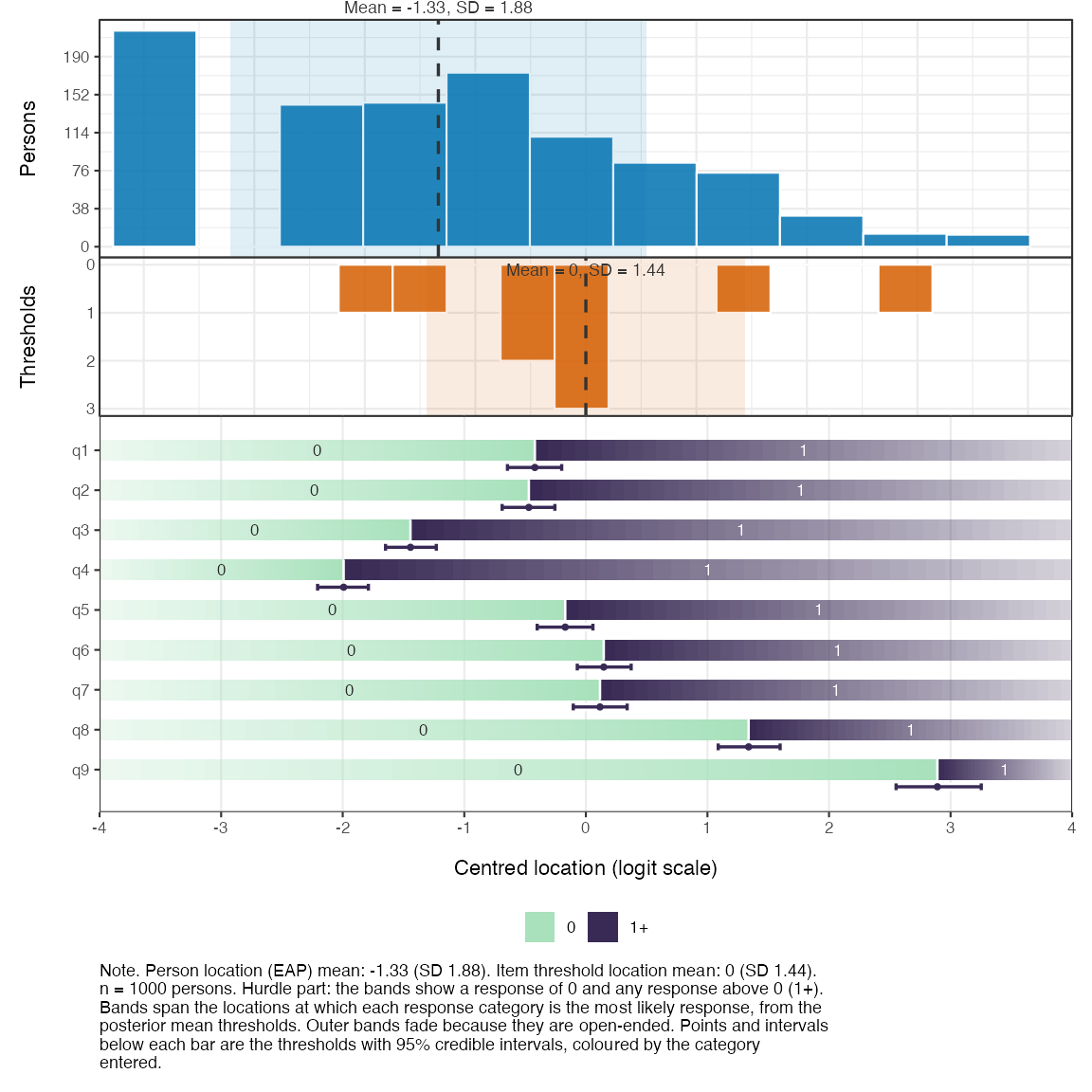

Figure 3. Targeting, hurdle submodel

targ$pcm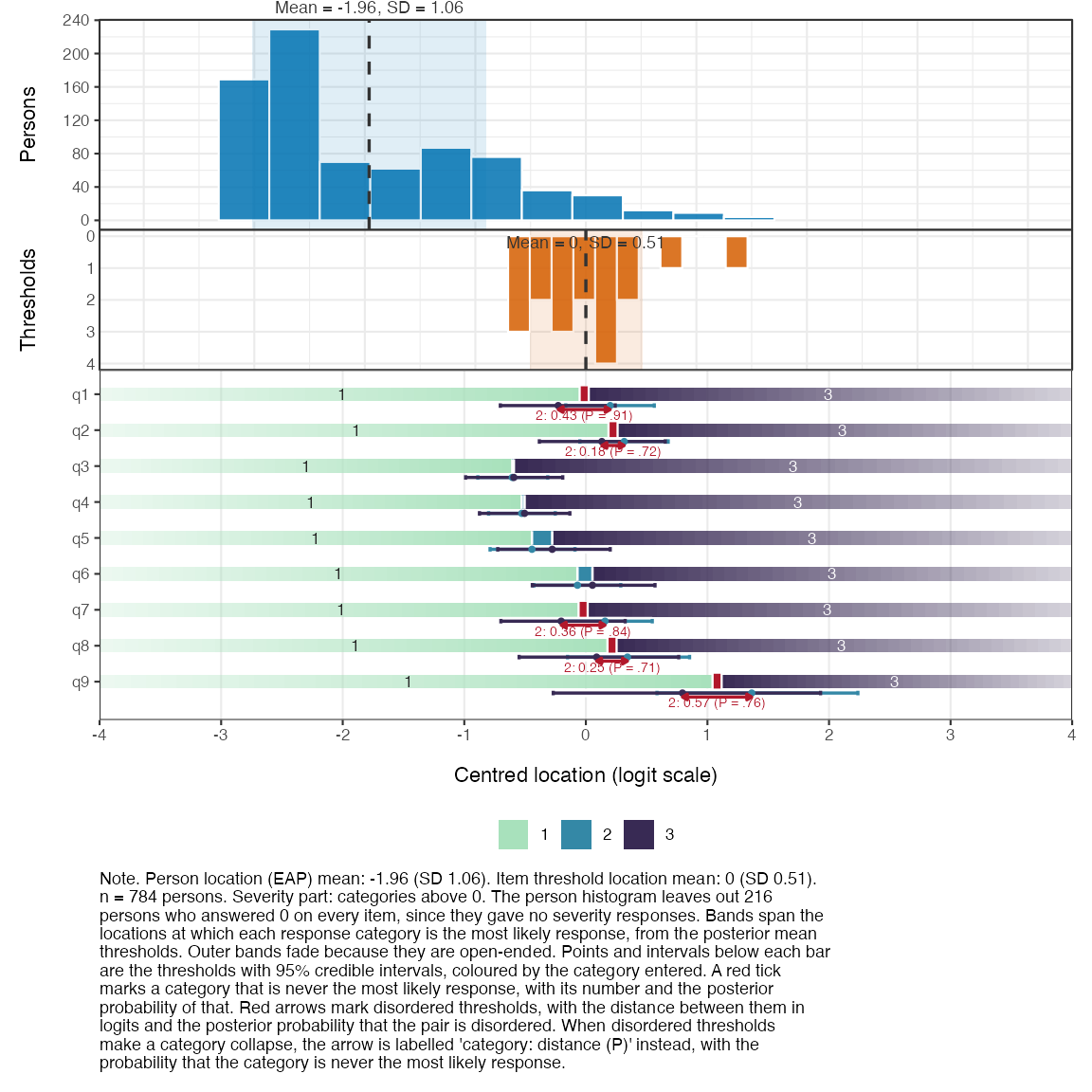

Figure 4. Targeting, severity submodel

In the hurdle plot, the item difficulties spread from about -2 to 3 and cover most of the persons. The persons who answered 0 on every item still form a spike at the low end, but the rest of the distribution is spread out, unlike in the PCM. The severity plot shows only the 784 persons with at least one response above 0. Their mean severity is about 2 logits below the mean threshold: most of those who report symptoms report them as occurring on “Several days”, so the severity thresholds are targeted above most of the sample. The category bands show the disordered severity thresholds from above: for q1, q2, q7, q8 and q9, category 2 is marked in red, with posterior probabilities from 0.71 to 0.91 that it is never the most likely response.

Item fit

infit_statistic_hpcm() computes posterior predictive infit for each submodel. The hurdle infit uses all responses, with 0 versus above 0 as the outcome. The severity infit uses only the responses above 0. Each part is summarised with infit_post().

infit_hpcm <- infit_statistic_hpcm(fit_hpcm, ndraws_use = 500)

infit_hu <- infit_post(infit_hpcm$hurdle)
infit_hu$summary
#> # A tibble: 9 × 4
#>   item  infit_obs infit_rep infit_ppp
#>   <chr>     <dbl>     <dbl>     <dbl>
#> 1 q1        0.915     1.00      0.04 
#> 2 q2        0.881     0.999     0.01 
#> 3 q3        1.20      0.998     1    
#> 4 q4        0.971     1.00      0.242
#> 5 q5        1.12      0.996     0.988
#> 6 q6        0.922     0.997     0.1  
#> 7 q7        1.02      1.00      0.606
#> 8 q8        1.06      0.995     0.804
#> 9 q9        0.914     0.997     0.256
infit_hu$plot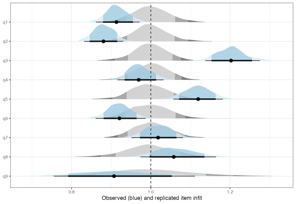

Figure 5. Infit, hurdle submodel

infit_sev <- infit_post(infit_hpcm$pcm)
infit_sev$summary
#> # A tibble: 9 × 4
#>   item  infit_obs infit_rep infit_ppp
#>   <chr>     <dbl>     <dbl>     <dbl>
#> 1 q1        1.02      1.00      0.58 
#> 2 q2        0.912     1.01      0.21 
#> 3 q3        1.02      0.997     0.632
#> 4 q4        0.984     1.00      0.406
#> 5 q5        1.03      1.00      0.614
#> 6 q6        0.949     0.996     0.334
#> 7 q7        1.04      1.00      0.618
#> 8 q8        1.15      0.999     0.834
#> 9 q9        1.16      1.01      0.68
infit_sev$plot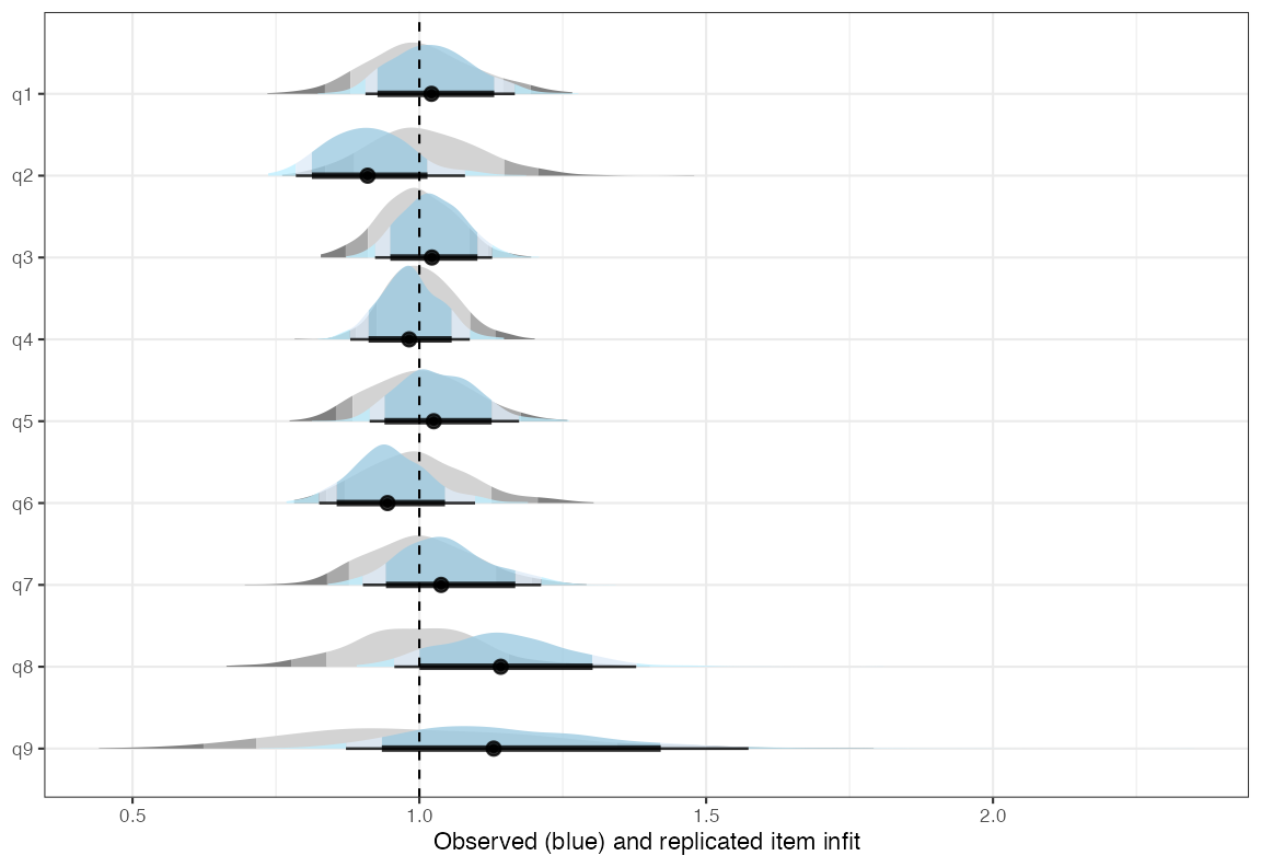

Figure 6. Infit, severity submodel

Unlike infit_statistic() for Rasch models, these expected values use the person locations in each posterior draw, not the total score. The total score is not sufficient for the person locations in the hurdle model, so the conditional method does not apply. Since the person locations are estimated from the same data, the posterior predictive p-values are conservative: values near 0 or 1 occur less often than they should when an item misfits. For the same reason, item_restscore_statistic() is not available for the hurdle model.

The conditional item characteristic curves show where along each latent variable the observed responses depart from the model.

icc <- plot_icc_hpcm(fit_hpcm, class_intervals = 3)
icc$hurdle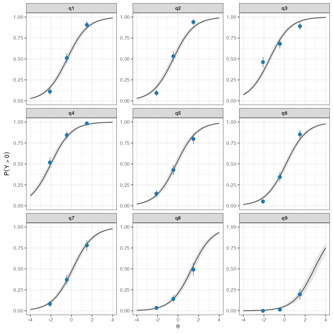

Figure 7. Conditional ICC, hurdle submodel

icc$pcm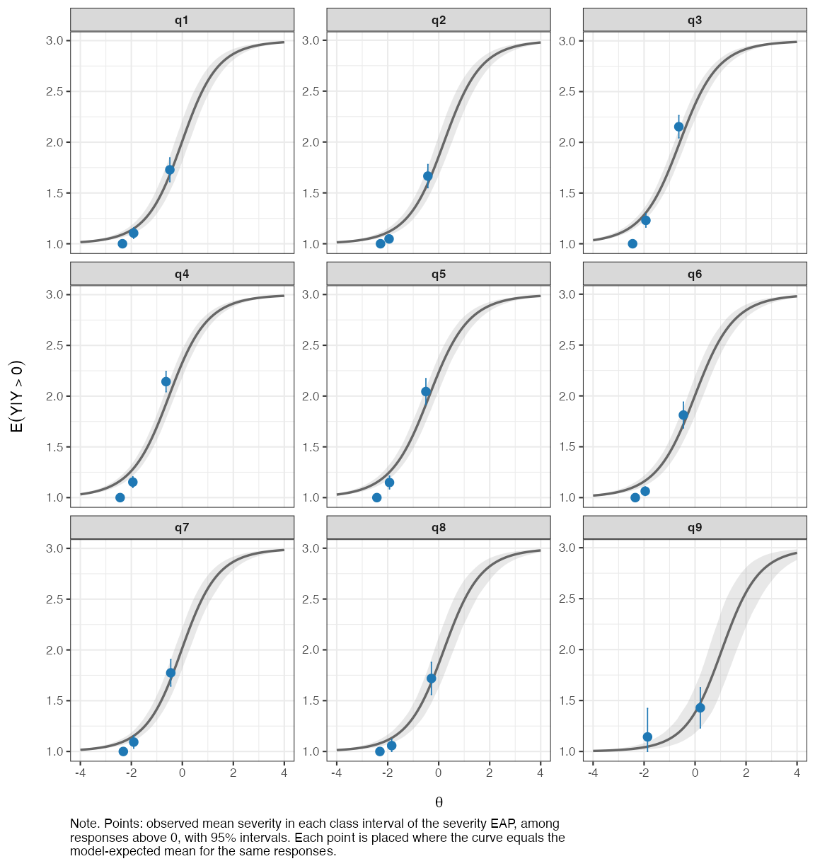

Figure 8. Conditional ICC, severity submodel

Three class intervals are used here, since with more intervals several severity points fall at the floor and overlap. In the hurdle panel, q3 is flatter than the model curve: people low on the presence trait report sleep problems more often than expected, which matches its infit above 1. q2 is steeper than the curve, matching its infit below 1.

In the severity panel, persons are grouped by their severity EAP, since the hurdle model has no sufficient sum score. EAPs are shrunk toward the mean, so each interval is placed where the curve equals the model’s expected mean for the same responses, and the observed points can be compared with the curve as in the other ICC plots. For several items, most clearly q3, q4 and q5, the observed mean is below the curve in the lowest interval and above it in the highest, so severity separates persons a little more than the model expects.

Local dependence

q3_statistic_hpcm() computes Yen’s Q3 residual correlations for each submodel, and q3_post() summarises them. As for infit, the residuals use the person locations in each draw.

q3_hpcm <- q3_statistic_hpcm(fit_hpcm, ndraws_use = 500)

q3_hu <- q3_post(q3_hpcm$hurdle)
q3_hu$summary
#> # A tibble: 36 × 8
#>    item_pair item_1 item_2 q3_obs q3_rep q3_diff q3_ppp q3_p_adj
#>    <chr>     <chr>  <chr>   <dbl>  <dbl>   <dbl>  <dbl>    <dbl>
#>  1 q2 : q6   q2     q6      0.303 -0.002   0.305  1        0    
#>  2 q1 : q2   q1     q2      0.193  0       0.193  1        0    
#>  3 q1 : q6   q1     q6      0.088 -0.001   0.089  0.98     0.25 
#>  4 q2 : q9   q2     q9      0.089  0       0.089  0.996    0.056
#>  5 q6 : q9   q6     q9      0.073 -0.001   0.075  0.98     0.412
#>  6 q7 : q8   q7     q8      0.073 -0.001   0.075  0.964    0.468
#>  7 q3 : q4   q3     q4      0.071 -0.001   0.072  0.962    0.578
#>  8 q5 : q7   q5     q7      0.057  0.001   0.056  0.916    0.868
#>  9 q4 : q6   q4     q6      0.031 -0.001   0.032  0.832    0.996
#> 10 q1 : q9   q1     q9      0.031  0.002   0.029  0.81     1    
#> # ℹ 26 more rows
q3_hu$plot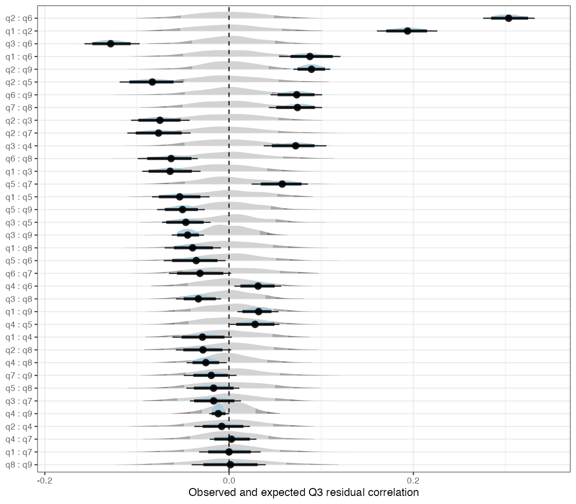

Figure 9. Q3, hurdle submodel

q3_sev <- q3_post(q3_hpcm$pcm)
q3_sev$summary
#> # A tibble: 36 × 8
#>    item_pair item_1 item_2 q3_obs q3_rep q3_diff q3_ppp q3_p_adj
#>    <chr>     <chr>  <chr>   <dbl>  <dbl>   <dbl>  <dbl>    <dbl>
#>  1 q1 : q2   q1     q2      0.279  0.001   0.278  1        0.004
#>  2 q2 : q6   q2     q6      0.195  0.002   0.193  0.994    0.148
#>  3 q8 : q9   q8     q9      0.182  0.002   0.181  0.818    0.998
#>  4 q5 : q6   q5     q6      0.162  0.004   0.158  0.964    0.614
#>  5 q3 : q4   q3     q4      0.133  0       0.133  0.98     0.352
#>  6 q7 : q9   q7     q9      0.115 -0.003   0.118  0.788    1    
#>  7 q6 : q7   q6     q7      0.1   -0.004   0.104  0.84     0.996
#>  8 q3 : q8   q3     q8      0.056  0.001   0.055  0.684    1    
#>  9 q1 : q7   q1     q7      0.032 -0.005   0.037  0.658    1    
#> 10 q4 : q5   q4     q5      0.033 -0.001   0.034  0.658    1    
#> # ℹ 26 more rows
q3_sev$plot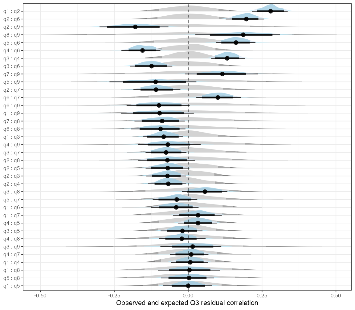

Figure 10. Q3, severity submodel

The largest residual correlations involve q1 (little interest), q2 (feeling down) and q6 (feeling bad about yourself), in both submodels. Q3 is about 0.30 for q2 and q6 in the hurdle submodel and about 0.28 for q1 and q2 in the severity submodel. These three items share more than the model allows, in whether they are reported and in how often.

Presence and severity compared

Splitting the model in two shows where the misfit of the PCM comes from.

• Item fit. The flagged misfit is in the hurdle part: q3 (sleep) and q5 (appetite) underfit, and q2 and q1 overfit. The overfitting items are the ones in the strongest dependent pairs below, and that dependence also makes the other items look more underfit, so the pattern says more about the mood items than about sleep or appetite as such. In the severity part, the ppp ranges from 0.21 to 0.83, with the highest infit for q8 and q9 (about 1.15), and nothing is flagged.
• Local dependence. The core mood items depend on each other in both parts. In the hurdle part, two pairs are flagged after adjustment for the 36 pairs, q2 with q6 (q3_diff 0.31) and q1 with q2 (0.19), and the next largest difference is 0.09. In the severity part, q1 with q2 is the only flagged pair (0.28, q3_p_adj .004), but six more pairs have differences from 0.10 to 0.19, including q8 with q9, q5 with q6 and q3 with q4. Their q3_ppp values range from 0.79 to 0.99, so these differences are uncertain. If they are real, which symptoms occur together frequently is less well described by one severity trait than which symptoms occur at all.

Both comparisons need care. The severity part uses only the responses above 0, about a third of all responses here, and 37% of those with any such response have only one or two. Its statistics are much less certain, and with this sample it has little power to flag misfit or dependence. A severity part without flagged items is therefore weak evidence that it fits. The posterior predictive p-values in both parts are also conservative.

Why would the two parts differ? Watts et al. (2026) found that broad dimensions of psychopathology are strongly associated among people with few or no symptoms and only weakly among people with more symptoms. Much of the covariation between the dimensions thus came from people with few or no symptoms. If the same holds for the items of one scale, people with few or no symptoms would account for much of the association between items in the hurdle part, which models whether each symptom is present. Among those who report a symptom, how often it occurs would depend more on the particular symptom, which would show as more residual dependence in the severity part. That would fit the pattern above, but other explanations fit it too, and this example was not set up to tell them apart. The additional dependence in the severity part rests on pairs whose differences are uncertain, because that part has little information. It also uses only responses above 0, and that selection by itself can change how strongly the items are associated. A more direct check would compare residual correlations between groups of persons at different levels of symptom presence, which needs a larger sample than this one.

Person locations and reliability

ppar <- person_parameters_hpcm(fit_hpcm, draws = TRUE)
head(ppar$hurdle$person_estimates)
#> # A tibble: 6 × 7
#>   id    n_items sum_score   eap eap_se   wle wle_se
#>   <chr>   <int>     <int> <dbl>  <dbl> <dbl>  <dbl>
#> 1 1           9         1 -2.62  0.992 -2.32  1.03 
#> 2 2           9         2 -1.84  0.856 -1.54  0.859
#> 3 3           9         1 -2.60  0.968 -2.32  1.03 
#> 4 4           9         9  3.62  1.11   4.13  1.82 
#> 5 5           9         8  2.07  0.865  2.47  1.14 
#> 6 6           9         0 -3.87  1.30  -3.68  1.64
head(ppar$pcm$person_estimates)
#> # A tibble: 6 × 5
#>   id    sum_score n_active    eap eap_se
#>   <chr>     <int>    <int>  <dbl>  <dbl>
#> 1 1             1        1 -3.08   1.10 
#> 2 2             2        2 -2.92   0.979
#> 3 3             1        1 -2.98   1.14 
#> 4 4            24        9  1.12   0.524
#> 5 5            14        8 -0.589  0.454
#> 6 6             0        0 -3.41   1.25

Each person gets a hurdle location (with EAP and WLE) and a severity location (EAP only). The severity location of a person who answered 0 on every item rests on the prior and on the correlation with the hurdle location only, since that person gave no severity responses.

rel <- RMUreliability_hpcm(ppar)
rel$hurdle
#>   rmu_estimate hdci_lowerbound hdci_upperbound .width .point .interval
#> 1    0.7955721       0.7754342       0.8134001   0.95   mean      hdci
rel$pcm
#>   rmu_estimate hdci_lowerbound hdci_upperbound .width .point .interval
#> 1    0.5777624       0.5348526        0.625631   0.95   mean      hdci

Reliability is computed per submodel with relative measurement uncertainty (Bignardi et al. 2026). For comparison, the RMU reliability of the PCM:

person_draws_pcm <- fit_pcm %>%
  as_draws_df() %>%
  as_tibble() %>%
  select(starts_with("r_id")) %>%
  t()
RMUreliability(person_draws_pcm)
#>   rmu_estimate hdci_lowerbound hdci_upperbound .width .point .interval
#> 1    0.7882207       0.7680069       0.8095181   0.95   mean      hdci

The presence location is about as reliable as the PCM location (both about 0.80). The severity location is much less reliable (about 0.58), since it rests on the items each person endorsed, often one or two, and mostly on the lowest positive category.

Does the hurdle model fit better?

Both models describe the same responses, so they can be compared with approximate leave-one-out cross-validation. The PCM uses the response coded from 1, which shifts the category labels but not the probabilities.

loo_pcm  <- loo(fit_pcm)
loo_hpcm <- loo(fit_hpcm)
loo_compare(list(PCM = loo_pcm, hPCM = loo_hpcm))
#>  model elpd_diff se_diff p_worse diag_diff       diag_elpd
#>   hPCM       0.0     0.0      NA           31 k_psis > 0.7
#>    PCM    -218.2    20.6    1.00           19 k_psis > 0.7
#> 
#> Diagnostic flags present.
#> See ?`loo-glossary` (sections `diag_diff` and `diag_elpd`)
#> or https://mc-stan.org/loo/reference/loo-glossary.html.

loo_compare() warns that the two models do not have the same response variable, because the PCM response is coded from 1. The probabilities of the observed responses are the same, so the comparison is valid. We suppress the warning above.

# Share of Pareto k values above 0.7 (unreliable importance sampling)
mean(loo_pcm$diagnostics$pareto_k > 0.7)
#> [1] 0.002111111
mean(loo_hpcm$diagnostics$pareto_k > 0.7)
#> [1] 0.003444444

# Difference in expected log predictive density per item
elpd_diff <- loo_hpcm$pointwise[, "elpd_loo"] - loo_pcm$pointwise[, "elpd_loo"]
round(tapply(elpd_diff, fit_hpcm$data$item, sum), 1)
#>   q1   q2   q3   q4   q5   q6   q7   q8   q9 
#> 52.7 30.6 15.6 30.9 23.4 28.8 20.2 10.6  5.4

The hurdle PCM predicts held-out responses better, by about 218 in expected log predictive density (SE about 21). Fewer than 0.5% of the Pareto k values are above 0.7, so the approximation is reliable. The gain holds for every item, and is largest for q1 and smallest for q9, the item most people do not report at all.

References

Bignardi, Giacomo, Rogier Kievit, and Paul-Christian Bürkner. 2026. A General Method for Estimating Reliability Using Bayesian Measurement Uncertainty. OSF. https://osf.io/preprints/psyarxiv/h54k8.

Bürkner, Paul-Christian. 2021. “Bayesian Item Response Modeling in R with Brms and Stan.” Journal of Statistical Software 100: 1–54. https://doi.org/10.18637/jss.v100.i05.

Kroenke, Kurt, Robert L. Spitzer, and Janet B. W. Williams. 2001. “The PHQ-9: Validity of a Brief Depression Severity Measure.” Journal of General Internal Medicine 16 (9): 606–13. https://doi.org/10.1046/j.1525-1497.2001.016009606.x.

Magnus, Brooke E., and Mauricio Garnier-Villarreal. 2022. “A Multidimensional Zero-Inflated Graded Response Model for Ordinal Symptom Data.” Psychological Methods 27 (2): 261–79. https://doi.org/10.1037/met0000395.

Magnus, Brooke E., and Yang Liu. 2022. “Symptom Presence and Symptom Severity as Unique Indicators of Psychopathology: An Application of Multidimensional Zero-Inflated and Hurdle Graded Response Models.” Educational and Psychological Measurement 82 (5): 938–66. https://doi.org/10.1177/00131644211061820.

Watts, Ashley L., Adon F. G. Rosen, Ashley L. Greene, et al. 2026. “Covariation Among Higher-Order Psychopathology Dimensions Is Driven by Nomorbidity and Not Comorbidity.” Nature Mental Health 4: 1674–85. https://doi.org/10.1038/s44220-026-00727-0.