Rasch Partial Credit Model with easyRaschBayes
Source:vignettes/pcm-rasch-analysis.Rmd
pcm-rasch-analysis.RmdOverview
This vignette demonstrates a Partial Credit Model (PCM) Rasch
analysis workflow using easyRaschBayes. The analysis uses
the eRm::pcmdat2 dataset, a small polytomous item response
data set included in the eRm package.
All functions in this package work with a Bayesian brms
model object fitted with the acat (adjacent categories)
family, which parameterises the PCM. Dichotomous Rasch models can also
be fit using brms and analyzed with the functions in this
package. A code example is available here,
and more detail is available in Bürkner, 2021.
Below, there is some brief texts explaining the output and
interpretation of key functions. For a more extensive treatment of
various Rasch analysis aspects, please see the easyRasch
vignette. Also, each function includes documentation and example
code, use ?function in your console.
Data Preparation
library(easyRaschBayes)
library(brms)
library(dplyr)
library(tidyr)
library(tibble)
library(ggplot2)
eRm::pcmdat2 is in wide format with item responses coded
0, 1, 2, …. The brms acat family expects
response categories starting at 1, so we add 1 to every
response before reshaping to long format.
df_pcm <- eRm::pcmdat2 %>%
  mutate(across(everything(), ~ .x + 1)) %>%
  rownames_to_column("id") %>%
  pivot_longer(!id, # don't include the id variable in the wide->long transformation
               names_to = "item",
               values_to = "response")

head(df_pcm)
#> # A tibble: 6 × 3
#>   id    item  response
#>   <chr> <chr>    <dbl>
#> 1 1     I1           2
#> 2 1     I2           2
#> 3 1     I3           2
#> 4 1     I4           2
#> 5 2     I1           1
#> 6 2     I2           1
Visualizing response data
Before analyzing data, it is good to review the response distributions. There are three simple plotting functions included in the package. All make use of wide format datasets, where items are separate columns and respondents are rows.
plot_stackedbars(eRm::pcmdat2)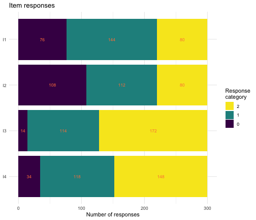
Stacked bars
The other two visualization functions are plot_tile()
and plot_bars()
Fitting the PCM
The model is fitted once and saved to disk. The code chunk below
shows the fitting call (not evaluated during R CMD check).
A pre-fitted model stored at fits/fit_pcm.rds is loaded
instead.
prior_pcm <- prior("normal(0, 3)", class = "Intercept") +
  prior("normal(0, 3)", class = "sd", group = "id")
fit_pcm <- brm(
  response | thres(gr = item) ~ 1 + (1 | id),
  data    = df_pcm,
  family  = acat,
  prior   = prior_pcm,
  chains  = 4,
  cores   = 4,
  iter    = 2000
)
saveRDS(fit_pcm, "fits/fit_pcm.rds")
fit_pcm <- readRDS("fits/fit_pcm.rds")Item Fit: Conditional Infit Statistics
infit_statistic() computes posterior predictive infit
(and outfit) statistics for each item. Values near 1.0 indicate good
fit; values above 1 suggest underfit (unexpected responses, often
indicating multidimensionality), values below 1 suggest overfit (too
predictable, often coinciding with local dependence issues).
The ndraws_use argument limits the number of posterior
draws used, which speeds up computation during exploration. For final
reporting, use all draws (set ndraws_use = NULL or omit
it).
fit_stats <- infit_statistic(fit_pcm, ndraws_use = 500)

# Post-process Infit
infit_results <- infit_post(fit_stats)
infit_results$summary
#> # A tibble: 4 × 4
#>   item  infit_obs infit_rep infit_ppp
#>   <chr>     <dbl>     <dbl>     <dbl>
#> 1 I1        1.04      1.00      0.292
#> 2 I2        1.08      1         0.11
#> 3 I3        0.917     1.00      0.89
#> 4 I4        1.03      0.999     0.364
infit_results$plot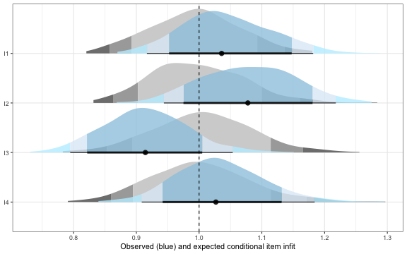
Conditional infit figure
infit_obs indicates the observed conditional infit,
which can be compared to infit_rep, which is akin to the
model expected value. Posterior predictive p-values (*_ppp)
close to 0.5 indicate that the observed statistic falls near the centre
of the posterior predictive distribution, implying good fit. Values near
0 or 1 warrant further investigation.
Item–Rest Score Association
item_restscore_statistic() computes Goodman-Kruskal’s
gamma between each item’s observed responses and the rest score (total
score minus the focal item). In a well-fitting Rasch model, gamma should
be positive and moderate and of similar magnitude for all items; high
values may indicate redundancy, low values suggest the item does not
relate well to the latent trait.
rest_stats <- item_restscore_statistic(fit_pcm, ndraws_use = 500)

rest_results <- item_restscore_post(rest_stats)
rest_results$summary
#> # A tibble: 4 × 5
#>   item  gamma_obs gamma_rep gamma_diff   ppp
#>   <chr>     <dbl>     <dbl>      <dbl> <dbl>
#> 1 I1        0.473     0.541     -0.068 0.118
#> 2 I2        0.441     0.543     -0.102 0.056
#> 3 I3        0.643     0.53       0.112 0.962
#> 4 I4        0.535     0.537     -0.002 0.492
rest_results$plot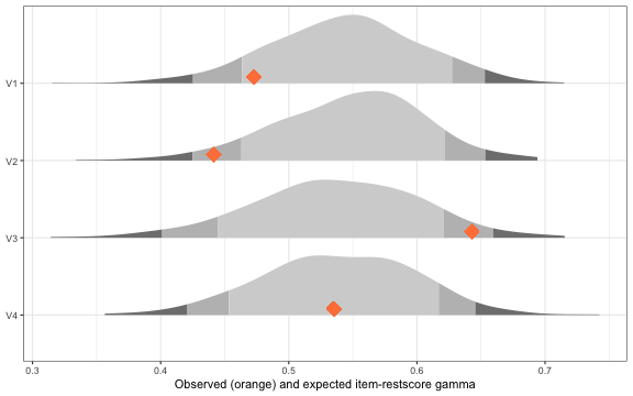
Item-restscore figure
Conditional ICC Plot
Shows item fit across the latent continuum, dividing the sample into n class intervals (default is 5).
plot_icc(fit_pcm)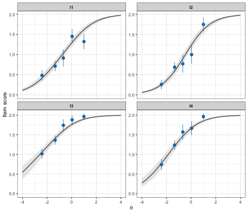
Conditional Item Characteristic Curves figure
Dimensionality: Residual PCA
plot_residual_pca() performs a principal components
analysis on the person-item residuals and plots the standardized
loadings on the first residual contrast factor together with item
locations and the uncertainty of both.
pca <- plot_residual_pca(fit_pcm, ndraws_use = 500)
pca$plot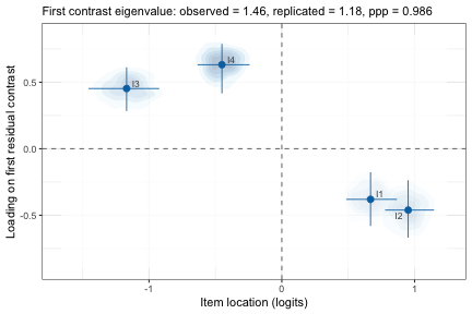
1st residual contrast loadings & locations
If the observed largest eigenvalue is smaller than the replicated, unidimensionality is supported. The ppp should not be close to 1.
Local Dependence: Q3 Residual Correlations
q3_statistic() computes Yen’s Q3 statistic — the
correlation between person-item residuals for every item pair. After
conditioning on the latent trait, residuals should be uncorrelated;
elevated Q3 values indicate local dependence (LD). Our primary metric
here is the ppp, that should not be close to 1.
q3_stats <- q3_statistic(fit_pcm, ndraws_use = 500)

q3_results <- q3_post(q3_stats)
q3_results$summary
#> # A tibble: 6 × 7
#>   item_pair item_1 item_2 q3_obs q3_rep q3_diff q3_ppp
#>   <chr>     <chr>  <chr>   <dbl>  <dbl>   <dbl>  <dbl>
#> 1 I3 : I4   I3     I4      0.34   0.001   0.339  1
#> 2 I1 : I2   I1     I2      0.102  0.002   0.1    0.994
#> 3 I1 : I3   I1     I3     -0.072 -0.004  -0.068  0.016
#> 4 I2 : I3   I2     I3     -0.088 -0.003  -0.085  0
#> 5 I1 : I4   I1     I4     -0.132  0      -0.132  0
#> 6 I2 : I4   I2     I4     -0.163 -0.002  -0.161  0
q3_results$plot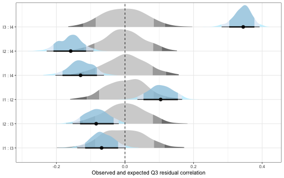
Q3 residual correlations
Item Category Probabilities
This plot shows the probability of using a response category on the y axis and the latent score on the x axis. The crossover points, where lines meet, are the item category threshold locations. Uncertainty is shown with the shaded area around each line.
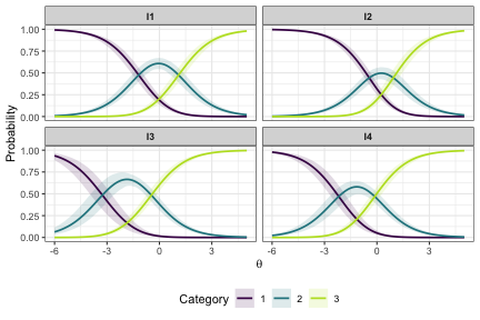
Item Probability Functions
Person–Item Targeting
plot_targeting() produces a Wright map (person–item
targeting plot) showing the distribution of person locations alongside
the item threshold locations on the same logit scale. Good targeting
occurs when person and item distributions overlap substantially.
plot_targeting(fit_pcm)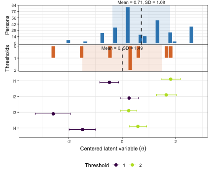
Targeting figure
Reliability: Relative Measurement Uncertainty
RMUreliability() provides a Bayesian reliability
estimate via Relative Measurement Uncertainty (RMU, see Bignardi et al.,
2025). It requires a matrix of person location draws with dimensions
.
The output is a point estimate and lower/upper 95% highest density
continuous intervals (HDCI).
person_draws <- fit_pcm %>%
  as_draws_df() %>%
  as_tibble() %>%
  select(starts_with("r_id")) %>%
  t()
rmu <- RMUreliability(person_draws)
rmu
#>   rmu_estimate hdci_lowerbound hdci_upperbound .width .point .interval
#> 1    0.6727799       0.6137229       0.7280385   0.95   mean      hdci
RMU values range from 0 to 1, with higher values indicating higher reliability, similarly to traditional reliability metrics such as Cronbach’s alpha.
Item Parameters
ipar <- item_parameters(fit_pcm)
knitr::kable(ipar$summary)| item | threshold | location | se | hdci_lower | hdci_upper | n_eff |
|---|---|---|---|---|---|---|
| I1 | 1 | -0.4792 | 0.1819 | -0.8505 | -0.1457 | 3734 |
| I1 | 2 | 1.8135 | 0.1840 | 1.4532 | 2.1753 | 3503 |
| I2 | 1 | 0.2591 | 0.1751 | -0.0743 | 0.6055 | 3423 |
| I2 | 2 | 1.6465 | 0.1908 | 1.3032 | 2.0377 | 3350 |
| I3 | 1 | -2.5798 | 0.3347 | -3.2377 | -1.9333 | 4000 |
| I3 | 2 | 0.2413 | 0.1569 | -0.0609 | 0.5475 | 3255 |
| I4 | 1 | -1.4880 | 0.2529 | -1.9889 | -1.0082 | 4000 |
| I4 | 2 | 0.5866 | 0.1608 | 0.2573 | 0.8902 | 4000 |
knitr::kable(ipar$locations_wide)| item | t1 | t2 | location |
|---|---|---|---|
| I3 | -2.5798 | 0.2413 | -1.1693 |
| I4 | -1.4880 | 0.5866 | -0.4507 |
| I1 | -0.4792 | 1.8135 | 0.6672 |
| I2 | 0.2591 | 1.6465 | 0.9528 |
Person Parameters
This estimates latent scores.
ppar <- person_parameters(fit_pcm)
knitr::kable(ppar$score_table)| sum_score | n | eap | eap_se | wle | wle_se |
|---|---|---|---|---|---|
| 0 | 7 | -1.9948 | 0.8723 | -7.0000 | NaN |
| 1 | 4 | -1.3413 | 0.7962 | -3.0165 | 1.3597 |
| 2 | 23 | -0.7713 | 0.7451 | -1.5860 | 0.9883 |
| 3 | 35 | -0.2446 | 0.7225 | -0.6911 | 0.8665 |
| 4 | 80 | 0.2582 | 0.7107 | 0.0616 | 0.8151 |
| 5 | 35 | 0.7609 | 0.7140 | 0.7901 | 0.8208 |
| 6 | 51 | 1.2865 | 0.7428 | 1.6205 | 0.9128 |
| 7 | 28 | 1.8658 | 0.8013 | 2.9849 | 1.3554 |
| 8 | 37 | 2.5625 | 0.8963 | 7.0000 | NaN |
hist(ppar$person_estimates$eap, col = "lightblue", main = "Histogram of EAP scores")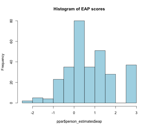
EAP score histogram
References
Bürkner, P.-C. (2021). Bayesian Item Response Modeling in R with brms and Stan. Journal of Statistical Software, 100, 1–54. https://doi.org/10.18637/jss.v100.i05
Bignardi, G., Kievit, R., & Bürkner, P.-C. (2025). A general method for estimating reliability using Bayesian Measurement Uncertainty. OSF. https://doi.org/10.31234/osf.io/h54k8_v1
Levy, R., Mislevy, R. J., & Sinharay, S. (2009). Posterior Predictive Model Checking for Multidimensionality in Item Response Theory. Applied Psychological Measurement, 33(7), 519–537. https://doi.org/10.1177/0146621608329504
Sinharay, S. (2006). Bayesian item fit analysis for unidimensional item response theory models. British Journal of Mathematical and Statistical Psychology, 59(2), 429–449. https://doi.org/10.1348/000711005X66888
Müller, M. (2020). Item fit statistics for Rasch analysis: Can we trust them? Journal of Statistical Distributions and Applications, 7(1), 5. https://doi.org/10.1186/s40488-020-00108-7
Kreiner, S. (2011). A Note on Item–Restscore Association in Rasch Models. Applied Psychological Measurement, 35(7), 557–561. https://doi.org/10.1177/0146621611410227