Psychometric analysis of the Mental Health Continuum-Short Form (MHC-SF)

Code

# one package below requires that you use devtools to install them manually:
# first install devtools by
# install.packages('devtools')

library(RISEkbmRasch) # devtools::install_github("pgmj/RISEkbmRasch")
library(lavaan)
library(lavaanPlot)
library(lavaanExtra)
library(readxl)
library(grateful)


### optional libraries
#library(TAM)
#library(skimr)

### some commands exist in multiple packages, here we define preferred ones that are frequently used
select <- dplyr::select
count <- dplyr::count
recode <- car::recode
rename <- dplyr::rename

source("RISE_theme.R")

Code

### other, bigger dataset from [@echeverría2017]
### read file
df.all <- read_excel("data/data_sMHCSF_Echeverria2017.xlsx")
df <- df.all
### create dif variables
dif.sex <- factor(df$Sex)
df$Sex <- NULL

### Load item information
# make sure that variable names in df match with itemlabels$itemnr
itemlabels <- read_excel("data/itemlabels_MHC_SF.xlsx") %>% 
  mutate(item = str_squish(item))

names(df) <- itemlabels$itemnr

df <- df %>%
  mutate(across(everything(), ~ car::recode(.x,"'Never'=0;'1 or 2 times a month'=1;'About 1 time a week'=2;'About 2 or 3 times a week'=3;'Almost daily'=4;'Daily'=5", as.factor = FALSE)))

3.1 Confirmatory factor analysis

Since the intended use of this scale is as a unidimensional scale, this is what we will primarily investigate.

The WLSMV estimator will be used, since we have ordinal data (Li 2016; Sellbom and Tellegen 2019).

We’ll use the lavaanExtra package to make things easier https://lavaanextra.remi-theriault.com/

Four fit indices will be in focus, apart from factor loadings.

RMSEA (should be below 0.06, but at least 0.10)
SRMR (below 0.08)
CFI and TLI (above 0.90 or ideally 0.95 (Hu and Bentler 1999).

Robust values for RMSEA och CFI/TLI are used, see https://lavaan.ugent.be/history/dot5.html#version-0.5-21, och a “scaled” value for chi2.

Recent developments in CFA propose that the old Hu & Bentler (1999) cutoff values should be replaced with dynamically set cutoffs (McNeish and Wolf 2021). They provide an online app: https://dynamicfit.app/

3.2 CFA 1

itemnr	item
mhc1	Happy
mhc2	Interested in life
mhc3	Satisfied with your life
mhc4	That you had something important to contribute to society?
mhc5	That you belonged to a community?
mhc6	That our society is becoming a better place for people like you?
mhc7	That people are basically good?
mhc8	That the way our society works makes sense to you?
mhc9	That you liked most parts of your personality?
mhc10	Good at managing the responsibilities of your daily life?
mhc11	That you had warm and trusting relationships with others?
mhc12	That you had experiences that challenged you to grow and become a better person?
mhc13	Confident to think or express your own ideas and opinions?
mhc14	That your life has a sense of direction or meaning to it?

Code

# Define latent variables
latent <- list(
  mhc = names(df)
)

# Write the model, and check it
cfa.model <- write_lavaan(latent = latent)
cat(cfa.model)

##################################################
# [-----Latent variables (measurement model)-----]

mhc =~ mhc1 + mhc2 + mhc3 + mhc4 + mhc5 + mhc6 + mhc7 + mhc8 + mhc9 + mhc10 + mhc11 + mhc12 + mhc13 + mhc14

Code

fit.cfa <- cfa(model = cfa.model, 
               data = df,
               estimator = "WLSMV",
               ordered = TRUE,
               rotation = "oblimin")
summary(fit.cfa)

lavaan 0.6.17 ended normally after 30 iterations

  Estimator                                       DWLS
  Optimization method                           NLMINB
  Number of model parameters                        84

  Number of observations                          3355

Model Test User Model:
                                              Standard      Scaled
  Test Statistic                              4169.805    6640.901
  Degrees of freedom                                77          77
  P-value (Chi-square)                           0.000       0.000
  Scaling correction factor                                  0.630
  Shift parameter                                           19.666
    simple second-order correction                                

Parameter Estimates:

  Parameterization                               Delta
  Standard errors                           Robust.sem
  Information                                 Expected
  Information saturated (h1) model        Unstructured

Latent Variables:
                   Estimate  Std.Err  z-value  P(>|z|)
  mhc =~                                              
    mhc1              1.000                           
    mhc2              1.097    0.013   83.955    0.000
    mhc3              1.096    0.012   88.245    0.000
    mhc4              0.931    0.015   62.942    0.000
    mhc5              0.827    0.016   50.640    0.000
    mhc6              1.013    0.014   70.135    0.000
    mhc7              0.892    0.015   59.932    0.000
    mhc8              0.964    0.015   66.353    0.000
    mhc9              1.062    0.013   82.216    0.000
    mhc10             1.018    0.014   74.679    0.000
    mhc11             1.062    0.013   81.047    0.000
    mhc12             1.075    0.013   82.817    0.000
    mhc13             1.042    0.014   76.416    0.000
    mhc14             1.158    0.013   87.275    0.000

Thresholds:
                   Estimate  Std.Err  z-value  P(>|z|)
    mhc1|t1          -2.214    0.058  -38.335    0.000
    mhc1|t2          -1.330    0.030  -43.952    0.000
    mhc1|t3          -0.775    0.024  -32.066    0.000
    mhc1|t4          -0.131    0.022   -6.023    0.000
    mhc1|t5           0.993    0.026   38.188    0.000
    mhc2|t1          -2.250    0.060  -37.635    0.000
    mhc2|t2          -1.536    0.034  -45.143    0.000
    mhc2|t3          -1.114    0.027  -40.800    0.000
    mhc2|t4          -0.641    0.023  -27.462    0.000
    mhc2|t5           0.089    0.022    4.091    0.000
    mhc3|t1          -1.755    0.039  -44.558    0.000
    mhc3|t2          -1.149    0.028  -41.452    0.000
    mhc3|t3          -0.762    0.024  -31.644    0.000
    mhc3|t4          -0.287    0.022  -13.084    0.000
    mhc3|t5           0.650    0.023   27.795    0.000
    mhc4|t1          -1.068    0.027  -39.876    0.000
    mhc4|t2          -0.553    0.023  -24.175    0.000
    mhc4|t3          -0.231    0.022  -10.573    0.000
    mhc4|t4           0.197    0.022    9.023    0.000
    mhc4|t5           0.952    0.026   37.177    0.000
    mhc5|t1          -0.611    0.023  -26.360    0.000
    mhc5|t2          -0.261    0.022  -11.915    0.000
    mhc5|t3          -0.018    0.022   -0.846    0.398
    mhc5|t4           0.303    0.022   13.771    0.000
    mhc5|t5           0.827    0.025   33.670    0.000
    mhc6|t1          -0.605    0.023  -26.125    0.000
    mhc6|t2          -0.038    0.022   -1.743    0.081
    mhc6|t3           0.316    0.022   14.355    0.000
    mhc6|t4           0.789    0.024   32.485    0.000
    mhc6|t5           1.573    0.035   45.173    0.000
    mhc7|t1          -1.324    0.030  -43.897    0.000
    mhc7|t2          -0.547    0.023  -23.938    0.000
    mhc7|t3          -0.162    0.022   -7.437    0.000
    mhc7|t4           0.349    0.022   15.762    0.000
    mhc7|t5           1.296    0.030   43.590    0.000
    mhc8|t1          -0.812    0.024  -33.223    0.000
    mhc8|t2          -0.186    0.022   -8.540    0.000
    mhc8|t3           0.153    0.022    7.023    0.000
    mhc8|t4           0.635    0.023   27.262    0.000
    mhc8|t5           1.416    0.032   44.665    0.000
    mhc9|t1          -1.656    0.037  -45.047    0.000
    mhc9|t2          -0.987    0.026  -38.041    0.000
    mhc9|t3          -0.612    0.023  -26.393    0.000
    mhc9|t4          -0.108    0.022   -4.988    0.000
    mhc9|t5           0.882    0.025   35.277    0.000
    mhc10|t1         -1.758    0.039  -44.535    0.000
    mhc10|t2         -1.113    0.027  -40.774    0.000
    mhc10|t3         -0.752    0.024  -31.319    0.000
    mhc10|t4         -0.236    0.022  -10.814    0.000
    mhc10|t5          0.642    0.023   27.496    0.000
    mhc11|t1         -1.902    0.044  -43.214    0.000
    mhc11|t2         -1.212    0.029  -42.481    0.000
    mhc11|t3         -0.821    0.025  -33.479    0.000
    mhc11|t4         -0.299    0.022  -13.600    0.000
    mhc11|t5          0.548    0.023   23.972    0.000
    mhc12|t1         -1.705    0.038  -44.850    0.000
    mhc12|t2         -1.035    0.026  -39.173    0.000
    mhc12|t3         -0.641    0.023  -27.462    0.000
    mhc12|t4         -0.159    0.022   -7.299    0.000
    mhc12|t5          0.589    0.023   25.521    0.000
    mhc13|t1         -1.683    0.037  -44.949    0.000
    mhc13|t2         -1.096    0.027  -40.452    0.000
    mhc13|t3         -0.730    0.024  -30.569    0.000
    mhc13|t4         -0.272    0.022  -12.396    0.000
    mhc13|t5          0.482    0.023   21.363    0.000
    mhc14|t1         -1.526    0.034  -45.126    0.000
    mhc14|t2         -0.951    0.026  -37.147    0.000
    mhc14|t3         -0.680    0.024  -28.857    0.000
    mhc14|t4         -0.340    0.022  -15.385    0.000
    mhc14|t5          0.297    0.022   13.497    0.000

Variances:
                   Estimate  Std.Err  z-value  P(>|z|)
   .mhc1              0.454                           
   .mhc2              0.342                           
   .mhc3              0.344                           
   .mhc4              0.527                           
   .mhc5              0.627                           
   .mhc6              0.440                           
   .mhc7              0.565                           
   .mhc8              0.492                           
   .mhc9              0.384                           
   .mhc10             0.434                           
   .mhc11             0.384                           
   .mhc12             0.369                           
   .mhc13             0.408                           
   .mhc14             0.268                           
    mhc               0.546    0.012   46.175    0.000

Code

# create table with model fit metrics
# define fit metrics of interest

fit_metrics_robust <- c("chisq.scaled", "df", "pvalue.scaled", 
                         "cfi.robust", "tli.robust", "rmsea.robust", 
                        "rmsea.ci.lower.robust","rmsea.ci.upper.robust",
                        "srmr")

mfit1 <- 
  fitmeasures(fit.cfa, fit_metrics_robust) %>% 
  rbind() %>% 
  as.data.frame() %>% 
  mutate(across(where(is.numeric),~ round(.x, 3))) %>%
  rename(Chi2 = chisq.scaled,
         p = pvalue.scaled,
         CFI = cfi.robust,
         TLI = tli.robust,
         RMSEA = rmsea.robust,
         CI_low = rmsea.ci.lower.robust,
         CI_high = rmsea.ci.upper.robust,
         SRMR = srmr) %>% 
  add_column(Model = "Full 14 items", .before = "Chi2")

mfit1 %>% 
  kbl_rise()

	Model	Chi2	df	p	CFI	TLI	RMSEA	CI_low	CI_high	SRMR
.	Full 14 items	6640.901	77	0	0.834	0.804	0.147	0.143	0.151	0.075

Code

lavaanPlot(model = fit.cfa, 
           coefs = T, stand = T, covs = F,
           node_options = list(fontname = "Helvetica"), 
           edge_options = list(color = "grey"),
           graph_options = list(rankdir = "TD"))

Code

modificationIndices(fit.cfa,
                    standardized = T) %>% 
  as.data.frame(row.names = NULL) %>% 
  filter(mi > 30,
         op == "~~") %>% 
  arrange(desc(mi)) %>% 
  mutate(across(where(is.numeric),~ round(.x, 3))) %>%
  kbl_rise(fontsize = 14, tbl_width = 75)

lhs	op	rhs	mi	epc	sepc.lv	sepc.all	sepc.nox
mhc6	~~	mhc8	914.360	-0.293	-0.293	-0.630	-0.630
mhc7	~~	mhc8	560.583	-0.248	-0.248	-0.471	-0.471
mhc6	~~	mhc7	335.909	-0.204	-0.204	-0.409	-0.409
mhc2	~~	mhc3	255.671	-0.157	-0.157	-0.458	-0.458
mhc1	~~	mhc3	216.459	-0.151	-0.151	-0.383	-0.383
mhc9	~~	mhc13	177.391	-0.139	-0.139	-0.352	-0.352
mhc6	~~	mhc13	130.100	0.192	0.192	0.455	0.455
mhc8	~~	mhc13	129.068	0.188	0.188	0.420	0.420
mhc4	~~	mhc5	122.236	-0.149	-0.149	-0.259	-0.259
mhc11	~~	mhc12	116.336	-0.112	-0.112	-0.296	-0.296
mhc6	~~	mhc14	91.929	0.151	0.151	0.440	0.440
mhc6	~~	mhc9	88.970	0.141	0.141	0.343	0.343
mhc8	~~	mhc12	87.019	0.144	0.144	0.337	0.337
mhc1	~~	mhc2	86.332	-0.106	-0.106	-0.268	-0.268
mhc6	~~	mhc11	78.421	0.145	0.145	0.352	0.352
mhc9	~~	mhc10	78.369	-0.095	-0.095	-0.232	-0.232
mhc8	~~	mhc14	77.476	0.135	0.135	0.372	0.372
mhc7	~~	mhc14	76.694	0.139	0.139	0.357	0.357
mhc6	~~	mhc10	76.527	0.143	0.143	0.328	0.328
mhc8	~~	mhc11	75.639	0.136	0.136	0.312	0.312
mhc5	~~	mhc6	73.251	-0.114	-0.114	-0.217	-0.217
mhc6	~~	mhc12	70.251	0.128	0.128	0.319	0.319
mhc7	~~	mhc13	68.999	0.135	0.135	0.281	0.281
mhc3	~~	mhc6	68.486	0.125	0.125	0.320	0.320
mhc8	~~	mhc9	59.170	0.113	0.113	0.260	0.260
mhc7	~~	mhc12	54.474	0.112	0.112	0.246	0.246
mhc1	~~	mhc6	48.426	0.108	0.108	0.242	0.242
mhc1	~~	mhc8	48.316	0.110	0.110	0.233	0.233
mhc3	~~	mhc8	47.846	0.102	0.102	0.248	0.248
mhc7	~~	mhc10	44.892	0.107	0.107	0.215	0.215
mhc10	~~	mhc13	44.695	-0.077	-0.077	-0.184	-0.184
mhc8	~~	mhc10	44.412	0.105	0.105	0.227	0.227
mhc2	~~	mhc6	43.620	0.109	0.109	0.282	0.282
mhc5	~~	mhc10	43.281	0.113	0.113	0.217	0.217
mhc3	~~	mhc13	42.902	0.089	0.089	0.238	0.238
mhc2	~~	mhc8	40.921	0.108	0.108	0.264	0.264
mhc3	~~	mhc7	35.151	0.089	0.089	0.201	0.201
mhc13	~~	mhc14	34.932	-0.063	-0.063	-0.192	-0.192
mhc7	~~	mhc9	34.140	0.086	0.086	0.185	0.185
mhc12	~~	mhc13	30.691	-0.062	-0.062	-0.161	-0.161

Model fit is not good. Residual correlations are the likely cause. Items 3 and 6 are both in the top 4 MI with 2 correlations each, and we’ll remove those two and revise the model.

3.3 CFA 2

Code

removed.items <- c("mhc3","mhc6")
df2 <- df %>% 
  select(!any_of(removed.items))

itemnr	item
mhc1	Happy
mhc2	Interested in life
mhc4	That you had something important to contribute to society?
mhc5	That you belonged to a community?
mhc7	That people are basically good?
mhc8	That the way our society works makes sense to you?
mhc9	That you liked most parts of your personality?
mhc10	Good at managing the responsibilities of your daily life?
mhc11	That you had warm and trusting relationships with others?
mhc12	That you had experiences that challenged you to grow and become a better person?
mhc13	Confident to think or express your own ideas and opinions?
mhc14	That your life has a sense of direction or meaning to it?

Code

fit.cfa2 <- cfa(model = cfa.model2, 
                data = df2,
                estimator = "WLSMV",
                ordered = TRUE,
                rotation = "oblimin")
summary(fit.cfa2)

lavaan 0.6.17 ended normally after 29 iterations

  Estimator                                       DWLS
  Optimization method                           NLMINB
  Number of model parameters                        72

  Number of observations                          3355

Model Test User Model:
                                              Standard      Scaled
  Test Statistic                              1862.845    3512.950
  Degrees of freedom                                54          54
  P-value (Chi-square)                           0.000       0.000
  Scaling correction factor                                  0.531
  Shift parameter                                            8.055
    simple second-order correction                                

Parameter Estimates:

  Parameterization                               Delta
  Standard errors                           Robust.sem
  Information                                 Expected
  Information saturated (h1) model        Unstructured

Latent Variables:
                   Estimate  Std.Err  z-value  P(>|z|)
  mhc =~                                              
    mhc1              1.000                           
    mhc2              1.090    0.015   74.785    0.000
    mhc4              0.958    0.016   58.806    0.000
    mhc5              0.837    0.018   47.133    0.000
    mhc7              0.881    0.017   52.729    0.000
    mhc8              0.904    0.017   53.898    0.000
    mhc9              1.114    0.015   76.343    0.000
    mhc10             1.060    0.015   70.632    0.000
    mhc11             1.113    0.015   75.546    0.000
    mhc12             1.127    0.015   77.252    0.000
    mhc13             1.098    0.015   72.290    0.000
    mhc14             1.199    0.015   79.271    0.000

Thresholds:
                   Estimate  Std.Err  z-value  P(>|z|)
    mhc1|t1          -2.214    0.058  -38.335    0.000
    mhc1|t2          -1.330    0.030  -43.952    0.000
    mhc1|t3          -0.775    0.024  -32.066    0.000
    mhc1|t4          -0.131    0.022   -6.023    0.000
    mhc1|t5           0.993    0.026   38.188    0.000
    mhc2|t1          -2.250    0.060  -37.635    0.000
    mhc2|t2          -1.536    0.034  -45.143    0.000
    mhc2|t3          -1.114    0.027  -40.800    0.000
    mhc2|t4          -0.641    0.023  -27.462    0.000
    mhc2|t5           0.089    0.022    4.091    0.000
    mhc4|t1          -1.068    0.027  -39.876    0.000
    mhc4|t2          -0.553    0.023  -24.175    0.000
    mhc4|t3          -0.231    0.022  -10.573    0.000
    mhc4|t4           0.197    0.022    9.023    0.000
    mhc4|t5           0.952    0.026   37.177    0.000
    mhc5|t1          -0.611    0.023  -26.360    0.000
    mhc5|t2          -0.261    0.022  -11.915    0.000
    mhc5|t3          -0.018    0.022   -0.846    0.398
    mhc5|t4           0.303    0.022   13.771    0.000
    mhc5|t5           0.827    0.025   33.670    0.000
    mhc7|t1          -1.324    0.030  -43.897    0.000
    mhc7|t2          -0.547    0.023  -23.938    0.000
    mhc7|t3          -0.162    0.022   -7.437    0.000
    mhc7|t4           0.349    0.022   15.762    0.000
    mhc7|t5           1.296    0.030   43.590    0.000
    mhc8|t1          -0.812    0.024  -33.223    0.000
    mhc8|t2          -0.186    0.022   -8.540    0.000
    mhc8|t3           0.153    0.022    7.023    0.000
    mhc8|t4           0.635    0.023   27.262    0.000
    mhc8|t5           1.416    0.032   44.665    0.000
    mhc9|t1          -1.656    0.037  -45.047    0.000
    mhc9|t2          -0.987    0.026  -38.041    0.000
    mhc9|t3          -0.612    0.023  -26.393    0.000
    mhc9|t4          -0.108    0.022   -4.988    0.000
    mhc9|t5           0.882    0.025   35.277    0.000
    mhc10|t1         -1.758    0.039  -44.535    0.000
    mhc10|t2         -1.113    0.027  -40.774    0.000
    mhc10|t3         -0.752    0.024  -31.319    0.000
    mhc10|t4         -0.236    0.022  -10.814    0.000
    mhc10|t5          0.642    0.023   27.496    0.000
    mhc11|t1         -1.902    0.044  -43.214    0.000
    mhc11|t2         -1.212    0.029  -42.481    0.000
    mhc11|t3         -0.821    0.025  -33.479    0.000
    mhc11|t4         -0.299    0.022  -13.600    0.000
    mhc11|t5          0.548    0.023   23.972    0.000
    mhc12|t1         -1.705    0.038  -44.850    0.000
    mhc12|t2         -1.035    0.026  -39.173    0.000
    mhc12|t3         -0.641    0.023  -27.462    0.000
    mhc12|t4         -0.159    0.022   -7.299    0.000
    mhc12|t5          0.589    0.023   25.521    0.000
    mhc13|t1         -1.683    0.037  -44.949    0.000
    mhc13|t2         -1.096    0.027  -40.452    0.000
    mhc13|t3         -0.730    0.024  -30.569    0.000
    mhc13|t4         -0.272    0.022  -12.396    0.000
    mhc13|t5          0.482    0.023   21.363    0.000
    mhc14|t1         -1.526    0.034  -45.126    0.000
    mhc14|t2         -0.951    0.026  -37.147    0.000
    mhc14|t3         -0.680    0.024  -28.857    0.000
    mhc14|t4         -0.340    0.022  -15.385    0.000
    mhc14|t5          0.297    0.022   13.497    0.000

Variances:
                   Estimate  Std.Err  z-value  P(>|z|)
   .mhc1              0.483                           
   .mhc2              0.385                           
   .mhc4              0.526                           
   .mhc5              0.638                           
   .mhc7              0.598                           
   .mhc8              0.577                           
   .mhc9              0.358                           
   .mhc10             0.419                           
   .mhc11             0.359                           
   .mhc12             0.344                           
   .mhc13             0.377                           
   .mhc14             0.257                           
    mhc               0.517    0.013   41.067    0.000

Code

# create table with model fit metrics

mfit2 <- 
  fitmeasures(fit.cfa2, fit_metrics_robust) %>% 
  rbind() %>% 
  as.data.frame() %>% 
  mutate(across(where(is.numeric),~ round(.x, 3))) %>%
  rename(Chi2 = chisq.scaled,
         p = pvalue.scaled,
         CFI = cfi.robust,
         TLI = tli.robust,
         RMSEA = rmsea.robust,
         CI_low = rmsea.ci.lower.robust,
         CI_high = rmsea.ci.upper.robust,
         SRMR = srmr)  %>% 
  add_column(Model = "3 and 6 removed", .before = "Chi2")

rbind(mfit1,mfit2) %>%
  remove_rownames() %>% 
  kbl_rise()

Model	Chi2	df	p	CFI	TLI	RMSEA	CI_low	CI_high	SRMR
Full 14 items	6640.901	77	0	0.834	0.804	0.147	0.143	0.151	0.075
3 and 6 removed	3512.950	54	0	0.896	0.873	0.123	0.118	0.127	0.057

Code

lavaanPlot(model = fit.cfa2, 
           coefs = T, stand = T, covs = F,
           node_options = list(fontname = "Helvetica"), 
           edge_options = list(color = "grey"),
           graph_options = list(rankdir = "TD"))

Code

modificationIndices(fit.cfa2,
                    standardized = T) %>% 
  as.data.frame(row.names = NULL) %>% 
  filter(mi > 30,
         op == "~~") %>% 
  arrange(desc(mi)) %>% 
  mutate(across(where(is.numeric),~ round(.x, 3))) %>%
  kbl_rise(fontsize = 14, tbl_width = 75)

lhs	op	rhs	mi	epc	sepc.lv	sepc.all	sepc.nox
mhc7	~~	mhc8	997.804	-0.338	-0.338	-0.575	-0.575
mhc1	~~	mhc2	186.158	-0.159	-0.159	-0.370	-0.370
mhc4	~~	mhc5	137.381	-0.160	-0.160	-0.277	-0.277
mhc9	~~	mhc13	100.292	-0.108	-0.108	-0.296	-0.296
mhc8	~~	mhc13	83.460	0.153	0.153	0.328	0.328
mhc7	~~	mhc13	62.901	0.130	0.130	0.275	0.275
mhc11	~~	mhc12	60.513	-0.083	-0.083	-0.237	-0.237
mhc7	~~	mhc14	58.098	0.123	0.123	0.314	0.314
mhc7	~~	mhc12	45.287	0.104	0.104	0.230	0.230
mhc9	~~	mhc10	43.884	-0.073	-0.073	-0.189	-0.189
mhc5	~~	mhc10	43.620	0.115	0.115	0.223	0.223
mhc8	~~	mhc12	43.037	0.103	0.103	0.230	0.230
mhc8	~~	mhc11	35.843	0.095	0.095	0.208	0.208
mhc7	~~	mhc10	34.334	0.094	0.094	0.189	0.189

Better fit, but still not within acceptable metrics. Residual correlations remain problematic, with pairs 1 & 2 and 7 & 8 having the biggest issues. Leaning on factor loadings as a selection criterion, we’ll remove the item with lower loading.

3.4 CFA 3

Code

removed.items <- c("mhc3","mhc6","mhc1","mhc8")
df2 <- df %>% 
  select(!any_of(removed.items))

itemnr	item
mhc2	Interested in life
mhc4	That you had something important to contribute to society?
mhc5	That you belonged to a community?
mhc7	That people are basically good?
mhc9	That you liked most parts of your personality?
mhc10	Good at managing the responsibilities of your daily life?
mhc11	That you had warm and trusting relationships with others?
mhc12	That you had experiences that challenged you to grow and become a better person?
mhc13	Confident to think or express your own ideas and opinions?
mhc14	That your life has a sense of direction or meaning to it?

Code

fit.cfa3 <- cfa(model = cfa.model3, 
                data = df2,
                estimator = "WLSMV",
                ordered = TRUE,
                rotation = "oblimin")
summary(fit.cfa3)

lavaan 0.6.17 ended normally after 25 iterations

  Estimator                                       DWLS
  Optimization method                           NLMINB
  Number of model parameters                        60

  Number of observations                          3355

Model Test User Model:
                                              Standard      Scaled
  Test Statistic                               570.535    1230.595
  Degrees of freedom                                35          35
  P-value (Chi-square)                           0.000       0.000
  Scaling correction factor                                  0.465
  Shift parameter                                            3.153
    simple second-order correction                                

Parameter Estimates:

  Parameterization                               Delta
  Standard errors                           Robust.sem
  Information                                 Expected
  Information saturated (h1) model        Unstructured

Latent Variables:
                   Estimate  Std.Err  z-value  P(>|z|)
  mhc =~                                              
    mhc2              1.000                           
    mhc4              0.912    0.015   62.352    0.000
    mhc5              0.787    0.017   46.287    0.000
    mhc7              0.736    0.017   43.431    0.000
    mhc9              1.064    0.014   78.579    0.000
    mhc10             1.014    0.013   75.872    0.000
    mhc11             1.062    0.014   77.268    0.000
    mhc12             1.078    0.014   77.300    0.000
    mhc13             1.059    0.014   76.685    0.000
    mhc14             1.145    0.014   83.522    0.000

Thresholds:
                   Estimate  Std.Err  z-value  P(>|z|)
    mhc2|t1          -2.250    0.060  -37.635    0.000
    mhc2|t2          -1.536    0.034  -45.143    0.000
    mhc2|t3          -1.114    0.027  -40.800    0.000
    mhc2|t4          -0.641    0.023  -27.462    0.000
    mhc2|t5           0.089    0.022    4.091    0.000
    mhc4|t1          -1.068    0.027  -39.876    0.000
    mhc4|t2          -0.553    0.023  -24.175    0.000
    mhc4|t3          -0.231    0.022  -10.573    0.000
    mhc4|t4           0.197    0.022    9.023    0.000
    mhc4|t5           0.952    0.026   37.177    0.000
    mhc5|t1          -0.611    0.023  -26.360    0.000
    mhc5|t2          -0.261    0.022  -11.915    0.000
    mhc5|t3          -0.018    0.022   -0.846    0.398
    mhc5|t4           0.303    0.022   13.771    0.000
    mhc5|t5           0.827    0.025   33.670    0.000
    mhc7|t1          -1.324    0.030  -43.897    0.000
    mhc7|t2          -0.547    0.023  -23.938    0.000
    mhc7|t3          -0.162    0.022   -7.437    0.000
    mhc7|t4           0.349    0.022   15.762    0.000
    mhc7|t5           1.296    0.030   43.590    0.000
    mhc9|t1          -1.656    0.037  -45.047    0.000
    mhc9|t2          -0.987    0.026  -38.041    0.000
    mhc9|t3          -0.612    0.023  -26.393    0.000
    mhc9|t4          -0.108    0.022   -4.988    0.000
    mhc9|t5           0.882    0.025   35.277    0.000
    mhc10|t1         -1.758    0.039  -44.535    0.000
    mhc10|t2         -1.113    0.027  -40.774    0.000
    mhc10|t3         -0.752    0.024  -31.319    0.000
    mhc10|t4         -0.236    0.022  -10.814    0.000
    mhc10|t5          0.642    0.023   27.496    0.000
    mhc11|t1         -1.902    0.044  -43.214    0.000
    mhc11|t2         -1.212    0.029  -42.481    0.000
    mhc11|t3         -0.821    0.025  -33.479    0.000
    mhc11|t4         -0.299    0.022  -13.600    0.000
    mhc11|t5          0.548    0.023   23.972    0.000
    mhc12|t1         -1.705    0.038  -44.850    0.000
    mhc12|t2         -1.035    0.026  -39.173    0.000
    mhc12|t3         -0.641    0.023  -27.462    0.000
    mhc12|t4         -0.159    0.022   -7.299    0.000
    mhc12|t5          0.589    0.023   25.521    0.000
    mhc13|t1         -1.683    0.037  -44.949    0.000
    mhc13|t2         -1.096    0.027  -40.452    0.000
    mhc13|t3         -0.730    0.024  -30.569    0.000
    mhc13|t4         -0.272    0.022  -12.396    0.000
    mhc13|t5          0.482    0.023   21.363    0.000
    mhc14|t1         -1.526    0.034  -45.126    0.000
    mhc14|t2         -0.951    0.026  -37.147    0.000
    mhc14|t3         -0.680    0.024  -28.857    0.000
    mhc14|t4         -0.340    0.022  -15.385    0.000
    mhc14|t5          0.297    0.022   13.497    0.000

Variances:
                   Estimate  Std.Err  z-value  P(>|z|)
   .mhc2              0.424                           
   .mhc4              0.521                           
   .mhc5              0.644                           
   .mhc7              0.688                           
   .mhc9              0.347                           
   .mhc10             0.407                           
   .mhc11             0.350                           
   .mhc12             0.330                           
   .mhc13             0.353                           
   .mhc14             0.245                           
    mhc               0.576    0.014   42.527    0.000

Code

# create table with model fit metrics

mfit3 <- 
  fitmeasures(fit.cfa3, fit_metrics_robust) %>% 
  rbind() %>% 
  as.data.frame() %>% 
  mutate(across(where(is.numeric),~ round(.x, 3))) %>%
  rename(Chi2 = chisq.scaled,
         p = pvalue.scaled,
         CFI = cfi.robust,
         TLI = tli.robust,
         RMSEA = rmsea.robust,
         CI_low = rmsea.ci.lower.robust,
         CI_high = rmsea.ci.upper.robust,
         SRMR = srmr)  %>% 
  add_column(Model = "3,6,1,8 removed", .before = "Chi2")

rbind(mfit1,mfit2,mfit3) %>%
  remove_rownames() %>% 
  kbl_rise()

Model	Chi2	df	CFI	TLI	RMSEA	CI_low	CI_high	SRMR
Full 14 items	6640.901	77	0.834	0.804	0.147	0.143	0.151	0.075
3 and 6 removed	3512.950	54	0.896	0.873	0.123	0.118	0.127	0.057
3,6,1,8 removed	1230.595	35	0.942	0.925	0.103	0.098	0.108	0.042

Code

lavaanPlot(model = fit.cfa3, 
           coefs = T, stand = T, covs = F,
           node_options = list(fontname = "Helvetica"), 
           edge_options = list(color = "grey"),
           graph_options = list(rankdir = "TD"))

Code

modificationIndices(fit.cfa3,
                    standardized = T) %>% 
  as.data.frame(row.names = NULL) %>% 
  filter(mi > 5,
         op == "~~") %>% 
  arrange(desc(mi)) %>% 
  mutate(across(where(is.numeric),~ round(.x, 3))) %>%
  kbl_rise(fontsize = 14, tbl_width = 75)

lhs	op	rhs	mi	epc	sepc.lv	sepc.all	sepc.nox
mhc4	~~	mhc5	144.907	-0.168	-0.168	-0.290	-0.290
mhc9	~~	mhc13	64.646	-0.090	-0.090	-0.257	-0.257
mhc5	~~	mhc7	61.409	-0.121	-0.121	-0.181	-0.181
mhc5	~~	mhc10	45.430	0.119	0.119	0.232	0.232
mhc2	~~	mhc14	42.330	-0.079	-0.079	-0.245	-0.245
mhc11	~~	mhc12	41.680	-0.072	-0.072	-0.210	-0.210
mhc9	~~	mhc10	28.613	-0.061	-0.061	-0.162	-0.162
mhc5	~~	mhc13	28.359	0.093	0.093	0.194	0.194
mhc5	~~	mhc9	26.308	0.086	0.086	0.183	0.183
mhc4	~~	mhc13	24.812	0.076	0.076	0.177	0.177
mhc4	~~	mhc11	21.340	0.069	0.069	0.161	0.161
mhc7	~~	mhc13	19.804	0.074	0.074	0.150	0.150
mhc2	~~	mhc13	18.595	0.062	0.062	0.161	0.161
mhc4	~~	mhc10	18.491	0.065	0.065	0.142	0.142
mhc11	~~	mhc14	10.988	0.041	0.041	0.139	0.139
mhc7	~~	mhc14	10.785	0.054	0.054	0.131	0.131
mhc2	~~	mhc7	10.381	-0.052	-0.052	-0.096	-0.096
mhc9	~~	mhc14	10.201	0.038	0.038	0.130	0.130
mhc4	~~	mhc7	9.860	-0.048	-0.048	-0.080	-0.080
mhc4	~~	mhc9	9.505	0.043	0.043	0.102	0.102
mhc5	~~	mhc14	7.787	0.047	0.047	0.118	0.118
mhc2	~~	mhc9	7.580	0.039	0.039	0.102	0.102
mhc2	~~	mhc4	6.659	-0.039	-0.039	-0.082	-0.082
mhc7	~~	mhc12	6.415	0.040	0.040	0.083	0.083
mhc10	~~	mhc13	6.216	-0.030	-0.030	-0.080	-0.080
mhc2	~~	mhc12	6.166	0.035	0.035	0.092	0.092
mhc9	~~	mhc12	5.380	0.029	0.029	0.084	0.084

RMSEA still not quite there, but other metrics look pretty good. Residual correlation between items 4 and 5 is high, so we’ll remove item 5 (lower factor loading than item 4).

3.5 CFA 4

Code

removed.items <- c("mhc3","mhc6","mhc1","mhc8","mhc5")
df2 <- df %>% 
  select(!any_of(removed.items))

itemnr	item
mhc2	Interested in life
mhc4	That you had something important to contribute to society?
mhc7	That people are basically good?
mhc9	That you liked most parts of your personality?
mhc10	Good at managing the responsibilities of your daily life?
mhc11	That you had warm and trusting relationships with others?
mhc12	That you had experiences that challenged you to grow and become a better person?
mhc13	Confident to think or express your own ideas and opinions?
mhc14	That your life has a sense of direction or meaning to it?

Code

fit.cfa4 <- cfa(model = cfa.model4, 
                data = df2,
                estimator = "WLSMV",
                ordered = TRUE,
                rotation = "oblimin")
summary(fit.cfa4)

lavaan 0.6.17 ended normally after 25 iterations

  Estimator                                       DWLS
  Optimization method                           NLMINB
  Number of model parameters                        54

  Number of observations                          3355

Model Test User Model:
                                              Standard      Scaled
  Test Statistic                               281.987     668.682
  Degrees of freedom                                27          27
  P-value (Chi-square)                           0.000       0.000
  Scaling correction factor                                  0.423
  Shift parameter                                            1.724
    simple second-order correction                                

Parameter Estimates:

  Parameterization                               Delta
  Standard errors                           Robust.sem
  Information                                 Expected
  Information saturated (h1) model        Unstructured

Latent Variables:
                   Estimate  Std.Err  z-value  P(>|z|)
  mhc =~                                              
    mhc2              1.000                           
    mhc4              0.889    0.015   59.383    0.000
    mhc7              0.720    0.017   41.662    0.000
    mhc9              1.072    0.014   78.070    0.000
    mhc10             1.025    0.013   75.992    0.000
    mhc11             1.061    0.014   75.825    0.000
    mhc12             1.083    0.014   76.577    0.000
    mhc13             1.067    0.014   76.236    0.000
    mhc14             1.150    0.014   82.455    0.000

Thresholds:
                   Estimate  Std.Err  z-value  P(>|z|)
    mhc2|t1          -2.250    0.060  -37.635    0.000
    mhc2|t2          -1.536    0.034  -45.143    0.000
    mhc2|t3          -1.114    0.027  -40.800    0.000
    mhc2|t4          -0.641    0.023  -27.462    0.000
    mhc2|t5           0.089    0.022    4.091    0.000
    mhc4|t1          -1.068    0.027  -39.876    0.000
    mhc4|t2          -0.553    0.023  -24.175    0.000
    mhc4|t3          -0.231    0.022  -10.573    0.000
    mhc4|t4           0.197    0.022    9.023    0.000
    mhc4|t5           0.952    0.026   37.177    0.000
    mhc7|t1          -1.324    0.030  -43.897    0.000
    mhc7|t2          -0.547    0.023  -23.938    0.000
    mhc7|t3          -0.162    0.022   -7.437    0.000
    mhc7|t4           0.349    0.022   15.762    0.000
    mhc7|t5           1.296    0.030   43.590    0.000
    mhc9|t1          -1.656    0.037  -45.047    0.000
    mhc9|t2          -0.987    0.026  -38.041    0.000
    mhc9|t3          -0.612    0.023  -26.393    0.000
    mhc9|t4          -0.108    0.022   -4.988    0.000
    mhc9|t5           0.882    0.025   35.277    0.000
    mhc10|t1         -1.758    0.039  -44.535    0.000
    mhc10|t2         -1.113    0.027  -40.774    0.000
    mhc10|t3         -0.752    0.024  -31.319    0.000
    mhc10|t4         -0.236    0.022  -10.814    0.000
    mhc10|t5          0.642    0.023   27.496    0.000
    mhc11|t1         -1.902    0.044  -43.214    0.000
    mhc11|t2         -1.212    0.029  -42.481    0.000
    mhc11|t3         -0.821    0.025  -33.479    0.000
    mhc11|t4         -0.299    0.022  -13.600    0.000
    mhc11|t5          0.548    0.023   23.972    0.000
    mhc12|t1         -1.705    0.038  -44.850    0.000
    mhc12|t2         -1.035    0.026  -39.173    0.000
    mhc12|t3         -0.641    0.023  -27.462    0.000
    mhc12|t4         -0.159    0.022   -7.299    0.000
    mhc12|t5          0.589    0.023   25.521    0.000
    mhc13|t1         -1.683    0.037  -44.949    0.000
    mhc13|t2         -1.096    0.027  -40.452    0.000
    mhc13|t3         -0.730    0.024  -30.569    0.000
    mhc13|t4         -0.272    0.022  -12.396    0.000
    mhc13|t5          0.482    0.023   21.363    0.000
    mhc14|t1         -1.526    0.034  -45.126    0.000
    mhc14|t2         -0.951    0.026  -37.147    0.000
    mhc14|t3         -0.680    0.024  -28.857    0.000
    mhc14|t4         -0.340    0.022  -15.385    0.000
    mhc14|t5          0.297    0.022   13.497    0.000

Variances:
                   Estimate  Std.Err  z-value  P(>|z|)
   .mhc2              0.426                           
   .mhc4              0.547                           
   .mhc7              0.703                           
   .mhc9              0.340                           
   .mhc10             0.398                           
   .mhc11             0.354                           
   .mhc12             0.327                           
   .mhc13             0.346                           
   .mhc14             0.241                           
    mhc               0.574    0.014   42.098    0.000

Code

# create table with model fit metrics

mfit4 <- 
  fitmeasures(fit.cfa4, fit_metrics_robust) %>% 
  rbind() %>% 
  as.data.frame() %>% 
  mutate(across(where(is.numeric),~ round(.x, 3))) %>%
  rename(Chi2 = chisq.scaled,
         p = pvalue.scaled,
         CFI = cfi.robust,
         TLI = tli.robust,
         RMSEA = rmsea.robust,
         CI_low = rmsea.ci.lower.robust,
         CI_high = rmsea.ci.upper.robust,
         SRMR = srmr)  %>% 
  add_column(Model = "3,6,1,8,5 removed", .before = "Chi2")

rbind(mfit1,mfit2,mfit3,mfit4) %>%
  remove_rownames() %>% 
  kbl_rise()

Model	Chi2	df	CFI	TLI	RMSEA	CI_low	CI_high	SRMR
Full 14 items	6640.901	77	0.834	0.804	0.147	0.143	0.151	0.075
3 and 6 removed	3512.950	54	0.896	0.873	0.123	0.118	0.127	0.057
3,6,1,8 removed	1230.595	35	0.942	0.925	0.103	0.098	0.108	0.042
3,6,1,8,5 removed	668.682	27	0.962	0.950	0.090	0.084	0.096	0.030

Code

lavaanPlot(model = fit.cfa4, 
           coefs = T, stand = T, covs = F,
           node_options = list(fontname = "Helvetica"), 
           edge_options = list(color = "grey"),
           graph_options = list(rankdir = "TD"))

Code

modificationIndices(fit.cfa4,
                    standardized = T) %>% 
  as.data.frame(row.names = NULL) %>% 
  filter(mi > 5,
         op == "~~") %>% 
  arrange(desc(mi)) %>% 
  mutate(across(where(is.numeric),~ round(.x, 3))) %>%
  kbl_rise(fontsize = 14, tbl_width = 75)

lhs	op	rhs	mi	epc	sepc.lv	sepc.all	sepc.nox
mhc9	~~	mhc13	50.681	-0.081	-0.081	-0.235	-0.235
mhc11	~~	mhc12	42.839	-0.073	-0.073	-0.216	-0.216
mhc2	~~	mhc14	42.683	-0.080	-0.080	-0.250	-0.250
mhc4	~~	mhc7	21.514	-0.070	-0.070	-0.114	-0.114
mhc2	~~	mhc13	20.519	0.066	0.066	0.172	0.172
mhc9	~~	mhc10	18.482	-0.049	-0.049	-0.134	-0.134
mhc4	~~	mhc13	16.278	0.062	0.062	0.142	0.142
mhc2	~~	mhc7	16.079	-0.065	-0.065	-0.119	-0.119
mhc9	~~	mhc14	15.643	0.048	0.048	0.166	0.166
mhc7	~~	mhc13	15.278	0.065	0.065	0.133	0.133
mhc2	~~	mhc4	14.721	-0.058	-0.058	-0.120	-0.120
mhc4	~~	mhc10	12.214	0.053	0.053	0.115	0.115
mhc11	~~	mhc14	10.991	0.041	0.041	0.141	0.141
mhc4	~~	mhc11	10.605	0.049	0.049	0.111	0.111
mhc2	~~	mhc9	8.849	0.043	0.043	0.112	0.112
mhc9	~~	mhc12	8.800	0.037	0.037	0.110	0.110
mhc10	~~	mhc12	7.085	0.034	0.034	0.094	0.094
mhc4	~~	mhc12	6.792	-0.035	-0.035	-0.083	-0.083
mhc4	~~	mhc14	6.698	-0.036	-0.036	-0.098	-0.098
mhc7	~~	mhc14	6.522	0.042	0.042	0.102	0.102
mhc2	~~	mhc12	6.431	0.036	0.036	0.095	0.095

All metrics are looking quite good except for RMSEA. It is acceptable but would preferrably be lower.

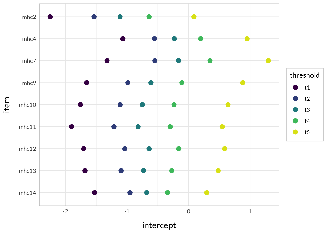
3.6 Intercepts?

Let’s have a look at the item intercepts.

Code

cfa.int4 <- 
  lavInspect(fit.cfa4, "wls.obs") %>% 
  as.data.frame() %>% 
  rownames_to_column("item_threshold") %>% 
  filter(!str_detect(item_threshold,"~~"))

names(cfa.int4)[2] <- "intercept"

cfa.int4 <- 
  cfa.int4 %>% 
  separate_wider_delim(item_threshold,
                       names = c("item","threshold"),
                       delim = "|")

cfa.int4 %>% 
  mutate(item = factor(item, rev(names(df2)))) %>% 
  ggplot(aes(y = item, x = intercept, color = threshold, group = item)) +
  geom_point(size = 3) +
  scale_color_viridis_d(end = 0.95)

Everything seems to be in order here. But then again, CFA assumes so.

3.7 CFA based on Rasch

Code

removed.items <- c("mhc3","mhc8","mhc5","mhc6","mhc7","mhc2")

df4 <- df %>% 
  select(!any_of(removed.items)) %>% 
  mutate(across(everything(), ~ car::recode(.x,"3=2;4=3;5=4"))) %>% 
  mutate(mhc4 = car::recode(mhc4,"1=0;2=1;3=2;4=3"))

itemnr	item
mhc1	Happy
mhc4	That you had something important to contribute to society?
mhc9	That you liked most parts of your personality?
mhc10	Good at managing the responsibilities of your daily life?
mhc11	That you had warm and trusting relationships with others?
mhc12	That you had experiences that challenged you to grow and become a better person?
mhc13	Confident to think or express your own ideas and opinions?
mhc14	That your life has a sense of direction or meaning to it?

Code

# Define latent variables
latent4 <- list(
  mhc = names(df4)
)

# Write the model, and check it
cfa.model4 <- write_lavaan(latent = latent4)

fit.cfa5 <- cfa(model = cfa.model4, 
                data = df4,
                estimator = "WLSMV",
                ordered = TRUE,
                rotation = "oblimin")
summary(fit.cfa5)

lavaan 0.6.17 ended normally after 17 iterations

  Estimator                                       DWLS
  Optimization method                           NLMINB
  Number of model parameters                        39

  Number of observations                          3355

Model Test User Model:
                                              Standard      Scaled
  Test Statistic                               146.247     347.347
  Degrees of freedom                                20          20
  P-value (Chi-square)                           0.000       0.000
  Scaling correction factor                                  0.422
  Shift parameter                                            0.822
    simple second-order correction                                

Parameter Estimates:

  Parameterization                               Delta
  Standard errors                           Robust.sem
  Information                                 Expected
  Information saturated (h1) model        Unstructured

Latent Variables:
                   Estimate  Std.Err  z-value  P(>|z|)
  mhc =~                                              
    mhc1              1.000                           
    mhc4              0.975    0.020   47.874    0.000
    mhc9              1.184    0.019   62.748    0.000
    mhc10             1.129    0.019   59.870    0.000
    mhc11             1.174    0.019   61.095    0.000
    mhc12             1.203    0.019   63.274    0.000
    mhc13             1.186    0.020   60.679    0.000
    mhc14             1.256    0.020   63.383    0.000

Thresholds:
                   Estimate  Std.Err  z-value  P(>|z|)
    mhc1|t1          -2.214    0.058  -38.335    0.000
    mhc1|t2          -1.330    0.030  -43.952    0.000
    mhc1|t3          -0.131    0.022   -6.023    0.000
    mhc1|t4           0.993    0.026   38.188    0.000
    mhc4|t1          -0.553    0.023  -24.175    0.000
    mhc4|t2           0.197    0.022    9.023    0.000
    mhc4|t3           0.952    0.026   37.177    0.000
    mhc9|t1          -1.656    0.037  -45.047    0.000
    mhc9|t2          -0.987    0.026  -38.041    0.000
    mhc9|t3          -0.108    0.022   -4.988    0.000
    mhc9|t4           0.882    0.025   35.277    0.000
    mhc10|t1         -1.758    0.039  -44.535    0.000
    mhc10|t2         -1.113    0.027  -40.774    0.000
    mhc10|t3         -0.236    0.022  -10.814    0.000
    mhc10|t4          0.642    0.023   27.496    0.000
    mhc11|t1         -1.902    0.044  -43.214    0.000
    mhc11|t2         -1.212    0.029  -42.481    0.000
    mhc11|t3         -0.299    0.022  -13.600    0.000
    mhc11|t4          0.548    0.023   23.972    0.000
    mhc12|t1         -1.705    0.038  -44.850    0.000
    mhc12|t2         -1.035    0.026  -39.173    0.000
    mhc12|t3         -0.159    0.022   -7.299    0.000
    mhc12|t4          0.589    0.023   25.521    0.000
    mhc13|t1         -1.683    0.037  -44.949    0.000
    mhc13|t2         -1.096    0.027  -40.452    0.000
    mhc13|t3         -0.272    0.022  -12.396    0.000
    mhc13|t4          0.482    0.023   21.363    0.000
    mhc14|t1         -1.526    0.034  -45.126    0.000
    mhc14|t2         -0.951    0.026  -37.147    0.000
    mhc14|t3         -0.340    0.022  -15.385    0.000
    mhc14|t4          0.297    0.022   13.497    0.000

Variances:
                   Estimate  Std.Err  z-value  P(>|z|)
   .mhc1              0.533                           
   .mhc4              0.556                           
   .mhc9              0.346                           
   .mhc10             0.405                           
   .mhc11             0.356                           
   .mhc12             0.325                           
   .mhc13             0.344                           
   .mhc14             0.263                           
    mhc               0.467    0.014   32.770    0.000

Code

# create table with model fit metrics

mfit5 <- 
  fitmeasures(fit.cfa5, fit_metrics_robust) %>% 
  rbind() %>% 
  as.data.frame() %>% 
  mutate(across(where(is.numeric),~ round(.x, 3))) %>%
  rename(Chi2 = chisq.scaled,
         p = pvalue.scaled,
         CFI = cfi.robust,
         TLI = tli.robust,
         RMSEA = rmsea.robust,
         CI_low = rmsea.ci.lower.robust,
         CI_high = rmsea.ci.upper.robust,
         SRMR = srmr)  %>% 
  add_column(Model = "Rasch based", .before = "Chi2")

rbind(mfit1,mfit2,mfit3,mfit4,mfit5) %>%
  remove_rownames() %>% 
  kbl_rise()

Model	Chi2	df	CFI	TLI	RMSEA	CI_low	CI_high	SRMR
Full 14 items	6640.901	77	0.834	0.804	0.147	0.143	0.151	0.075
3 and 6 removed	3512.950	54	0.896	0.873	0.123	0.118	0.127	0.057
3,6,1,8 removed	1230.595	35	0.942	0.925	0.103	0.098	0.108	0.042
3,6,1,8,5 removed	668.682	27	0.962	0.950	0.090	0.084	0.096	0.030
Rasch based	347.347	20	0.975	0.966	0.080	0.072	0.087	0.024

Code

lavaanPlot(model = fit.cfa5, 
           coefs = T, stand = T, covs = F,
           node_options = list(fontname = "Helvetica"), 
           edge_options = list(color = "grey"),
           graph_options = list(rankdir = "TD"))

Code

modificationIndices(fit.cfa5,
                    standardized = T) %>% 
  as.data.frame(row.names = NULL) %>% 
  filter(mi > 5,
         op == "~~") %>% 
  arrange(desc(mi)) %>% 
  mutate(across(where(is.numeric),~ round(.x, 3))) %>%
  kbl_rise(fontsize = 14, tbl_width = 75)

lhs	op	rhs	mi	epc	sepc.lv	sepc.all	sepc.nox
mhc9	~~	mhc13	36.071	-0.073	-0.073	-0.211	-0.211
mhc11	~~	mhc12	31.460	-0.067	-0.067	-0.197	-0.197
mhc1	~~	mhc13	16.674	0.065	0.065	0.152	0.152
mhc9	~~	mhc12	15.853	0.053	0.053	0.158	0.158
mhc4	~~	mhc14	14.461	-0.057	-0.057	-0.149	-0.149
mhc4	~~	mhc12	10.088	-0.047	-0.047	-0.110	-0.110
mhc9	~~	mhc10	9.935	-0.039	-0.039	-0.104	-0.104
mhc9	~~	mhc14	9.608	0.039	0.039	0.131	0.131
mhc10	~~	mhc12	9.382	0.041	0.041	0.113	0.113
mhc4	~~	mhc13	8.512	0.048	0.048	0.110	0.110
mhc4	~~	mhc11	7.582	0.045	0.045	0.100	0.100
mhc11	~~	mhc14	6.381	0.033	0.033	0.108	0.108
mhc4	~~	mhc10	6.125	0.041	0.041	0.086	0.086
mhc1	~~	mhc11	5.441	-0.033	-0.033	-0.077	-0.077

3.8 Software used

Code

pkgs <- cite_packages(cite.tidyverse = TRUE, 
                      output = "table",
                      bib.file = "grateful-refs.bib",
                      include.RStudio = TRUE,
                      out.dir = getwd())
formattable(pkgs, 
            table.attr = 'class=\"table table-striped\" style="font-size: 15px; font-family: Lato; width: 80%"')

Package	Version	Citation
base	4.3.2	R Core Team (2023)
car	3.1.2	Fox and Weisberg (2019)
cowplot	1.1.2	Wilke (2023)
eRm	1.0.4	Mair and Hatzinger (2007b); Mair and Hatzinger (2007a); Hatzinger and Rusch (2009); Rusch, Maier, and Hatzinger (2013); Koller, Maier, and Hatzinger (2015); Debelak and Koller (2019)
formattable	0.2.1	Ren and Russell (2021)
ggrepel	0.9.5	Slowikowski (2024)
glue	1.7.0	Hester and Bryan (2024)
kableExtra	1.3.4	Zhu (2021)
knitr	1.45	Xie (2014); Xie (2015); Xie (2023)
lavaan	0.6.17	Rosseel (2012)
lavaanExtra	0.2.0	Thériault (2023)
lavaanPlot	0.6.2	Lishinski (2021)
matrixStats	1.2.0	Bengtsson (2023)
mirt	1.41	Chalmers (2012)
mokken	3.1.0	Van der Ark (2007); Van der Ark (2012)
patchwork	1.2.0	Pedersen (2024)
psych	2.3.12	William Revelle (2023)
psychotree	0.16.0	Trepte and Verbeet (2010); Strobl, Wickelmaier, and Zeileis (2011); Strobl, Kopf, and Zeileis (2015); Komboz, Zeileis, and Strobl (2018); Wickelmaier and Zeileis (2018)
reshape	0.8.9	Wickham (2007)
RISEkbmRasch	0.1.31.0	Johansson (2024)
rmarkdown	2.25	Xie, Allaire, and Grolemund (2018); Xie, Dervieux, and Riederer (2020); Allaire et al. (2023)
tidyverse	2.0.0	Wickham et al. (2019)

3.9 References

Allaire, JJ, Yihui Xie, Christophe Dervieux, Jonathan McPherson, Javier Luraschi, Kevin Ushey, Aron Atkins, et al. 2023. rmarkdown: Dynamic Documents for r. https://github.com/rstudio/rmarkdown.

Bengtsson, Henrik. 2023. matrixStats: Functions That Apply to Rows and Columns of Matrices (and to Vectors). https://CRAN.R-project.org/package=matrixStats.

Chalmers, R. Philip. 2012. “mirt: A Multidimensional Item Response Theory Package for the R Environment.” Journal of Statistical Software 48 (6): 1–29. https://doi.org/10.18637/jss.v048.i06.

Debelak, Rudolf, and Ingrid Koller. 2019. “Testing the Local Independence Assumption of the Rasch Model with Q3-Based Nonparametric Model Tests.” Applied Psychological Measurement 44. https://doi.org/10.1177/0146621619835501.

Fox, John, and Sanford Weisberg. 2019. An R Companion to Applied Regression. Third. Thousand Oaks CA: Sage. https://socialsciences.mcmaster.ca/jfox/Books/Companion/.

Hatzinger, Reinhold, and Thomas Rusch. 2009. “IRT Models with Relaxed Assumptions in eRm: A Manual-Like Instruction.” Psychology Science Quarterly 51.

Hester, Jim, and Jennifer Bryan. 2024. glue: Interpreted String Literals. https://CRAN.R-project.org/package=glue.

Hu, Li-tze, and Peter M. Bentler. 1999. “Cutoff Criteria for Fit Indexes in Covariance Structure Analysis: Conventional Criteria Versus New Alternatives.” Structural Equation Modeling: A Multidisciplinary Journal 6 (1): 1–55. https://doi.org/10.1080/10705519909540118.

Johansson, Magnus. 2024. RISEkbmRasch: Psychometric Analysis in r with Rasch Measurement Theory. https://github.com/pgmj/RISEkbmRasch.

Koller, Ingrid, Marco Maier, and Reinhold Hatzinger. 2015. “An Empirical Power Analysis of Quasi-Exact Tests for the Rasch Model: Measurement Invariance in Small Samples.” Methodology 11. https://doi.org/10.1027/1614-2241/a000090.

Komboz, Basil, Achim Zeileis, and Carolin Strobl. 2018. “Tree-Based Global Model Tests for Polytomous Rasch Models.” Educational and Psychological Measurement 78 (1): 128–66. https://doi.org/10.1177/0013164416664394.

Li, Cheng-Hsien. 2016. “Confirmatory Factor Analysis with Ordinal Data: Comparing Robust Maximum Likelihood and Diagonally Weighted Least Squares.” Behavior Research Methods 48 (3): 936–49. https://doi.org/10.3758/s13428-015-0619-7.

Lishinski, Alex. 2021. lavaanPlot: Path Diagrams for “Lavaan” Models via “DiagrammeR”. https://CRAN.R-project.org/package=lavaanPlot.

Mair, Patrick, and Reinhold Hatzinger. 2007a. “CML Based Estimation of Extended Rasch Models with the eRm Package in r.” Psychology Science 49. https://doi.org/10.18637/jss.v020.i09.

———. 2007b. “Extended Rasch Modeling: The eRm Package for the Application of IRT Models in r.” Journal of Statistical Software 20. https://doi.org/10.18637/jss.v020.i09.

McNeish, Daniel, and Melissa G. Wolf. 2021. “Dynamic Fit Index Cutoffs for Confirmatory Factor Analysis Models.” Psychological Methods, October. https://doi.org/10.1037/met0000425.

Pedersen, Thomas Lin. 2024. patchwork: The Composer of Plots. https://CRAN.R-project.org/package=patchwork.

R Core Team. 2023. R: A Language and Environment for Statistical Computing. Vienna, Austria: R Foundation for Statistical Computing. https://www.R-project.org/.

Ren, Kun, and Kenton Russell. 2021. formattable: Create “Formattable” Data Structures. https://CRAN.R-project.org/package=formattable.

Rosseel, Yves. 2012. “lavaan: An R Package for Structural Equation Modeling.” Journal of Statistical Software 48 (2): 1–36. https://doi.org/10.18637/jss.v048.i02.

Rusch, Thomas, Marco Maier, and Reinhold Hatzinger. 2013. “Linear Logistic Models with Relaxed Assumptions in r.” In Algorithms from and for Nature and Life, edited by Berthold Lausen, Dirk van den Poel, and Alfred Ultsch. Studies in Classification, Data Analysis, and Knowledge Organization. New York: Springer. https://doi.org/10.1007/978-3-319-00035-0_34.

Sellbom, Martin, and Auke Tellegen. 2019. “Factor Analysis in Psychological Assessment Research: Common Pitfalls and Recommendations.” Psychological Assessment 31 (12): 1428–41. https://doi.org/10.1037/pas0000623.

Slowikowski, Kamil. 2024. ggrepel: Automatically Position Non-Overlapping Text Labels with “ggplot2”. https://CRAN.R-project.org/package=ggrepel.

Strobl, Carolin, Julia Kopf, and Achim Zeileis. 2015. “Rasch Trees: A New Method for Detecting Differential Item Functioning in the Rasch Model.” Psychometrika 80 (2): 289–316. https://doi.org/10.1007/s11336-013-9388-3.

Strobl, Carolin, Florian Wickelmaier, and Achim Zeileis. 2011. “Accounting for Individual Differences in Bradley-Terry Models by Means of Recursive Partitioning.” Journal of Educational and Behavioral Statistics 36 (2): 135–53. https://doi.org/10.3102/1076998609359791.

Thériault, Rémi. 2023. “lavaanExtra: Convenience Functions for Lavaan.” Journal of Open Source Software 8 (90): 5701. https://doi.org/10.21105/joss.05701.

Trepte, Sabine, and Markus Verbeet, eds. 2010. Allgemeinbildung in Deutschland – Erkenntnisse Aus Dem SPIEGEL Studentenpisa-Test. Wiesbaden: VS Verlag.

Van der Ark, L. Andries. 2007. “Mokken Scale Analysis in R.” Journal of Statistical Software 20 (11): 1–19. https://doi.org/10.18637/jss.v020.i11.

———. 2012. “New Developments in Mokken Scale Analysis in R.” Journal of Statistical Software 48 (5): 1–27. https://doi.org/10.18637/jss.v048.i05.

Wickelmaier, Florian, and Achim Zeileis. 2018. “Using Recursive Partitioning to Account for Parameter Heterogeneity in Multinomial Processing Tree Models.” Behavior Research Methods 50 (3): 1217–33. https://doi.org/10.3758/s13428-017-0937-z.

Wickham, Hadley. 2007. “Reshaping Data with the Reshape Package.” Journal of Statistical Software 21 (12). https://www.jstatsoft.org/v21/i12/.

Wickham, Hadley, Mara Averick, Jennifer Bryan, Winston Chang, Lucy D’Agostino McGowan, Romain François, Garrett Grolemund, et al. 2019. “Welcome to the tidyverse.” Journal of Open Source Software 4 (43): 1686. https://doi.org/10.21105/joss.01686.

Wilke, Claus O. 2023. cowplot: Streamlined Plot Theme and Plot Annotations for “ggplot2”. https://CRAN.R-project.org/package=cowplot.

William Revelle. 2023. psych: Procedures for Psychological, Psychometric, and Personality Research. Evanston, Illinois: Northwestern University. https://CRAN.R-project.org/package=psych.

Xie, Yihui. 2014. “knitr: A Comprehensive Tool for Reproducible Research in R.” In Implementing Reproducible Computational Research, edited by Victoria Stodden, Friedrich Leisch, and Roger D. Peng. Chapman; Hall/CRC.

———. 2015. Dynamic Documents with R and Knitr. 2nd ed. Boca Raton, Florida: Chapman; Hall/CRC. https://yihui.org/knitr/.

———. 2023. knitr: A General-Purpose Package for Dynamic Report Generation in r. https://yihui.org/knitr/.

Xie, Yihui, J. J. Allaire, and Garrett Grolemund. 2018. R Markdown: The Definitive Guide. Boca Raton, Florida: Chapman; Hall/CRC. https://bookdown.org/yihui/rmarkdown.

Xie, Yihui, Christophe Dervieux, and Emily Riederer. 2020. R Markdown Cookbook. Boca Raton, Florida: Chapman; Hall/CRC. https://bookdown.org/yihui/rmarkdown-cookbook.

Zhu, Hao. 2021. kableExtra: Construct Complex Table with “kable” and Pipe Syntax. https://CRAN.R-project.org/package=kableExtra.