5 GAD-7 – Return to work questionnaires

Code

library(tidyverse)
library(janitor)
library(skimr)
library(easyRasch)
library(haven)

source("ki.R")
theme_set(theme_ki())

### some commands exist in multiple packages, here we define preferred ones that are frequently used
select <- dplyr::select
count <- dplyr::count
recode <- car::recode
rename <- dplyr::rename

d.all <- read_spss("data/SUVRTW_LONG 240528 TOTAL.sav") 

d <- d.all %>% 
  select(starts_with("GAD7"),time) %>% 
  na.omit()

df <- d.all %>% 
  select(starts_with("GAD7"),time,PID) %>% 
  na.omit()

# subset and remove DIF variable(s)
dif.time <- d$time
d$time <- NULL

itemlabels <- read_csv("data/spss_labels.csv") %>% 
  filter(str_detect(itemnr,"GAD"))

5.1 Background

We have longitudinal data from 10 measurements.

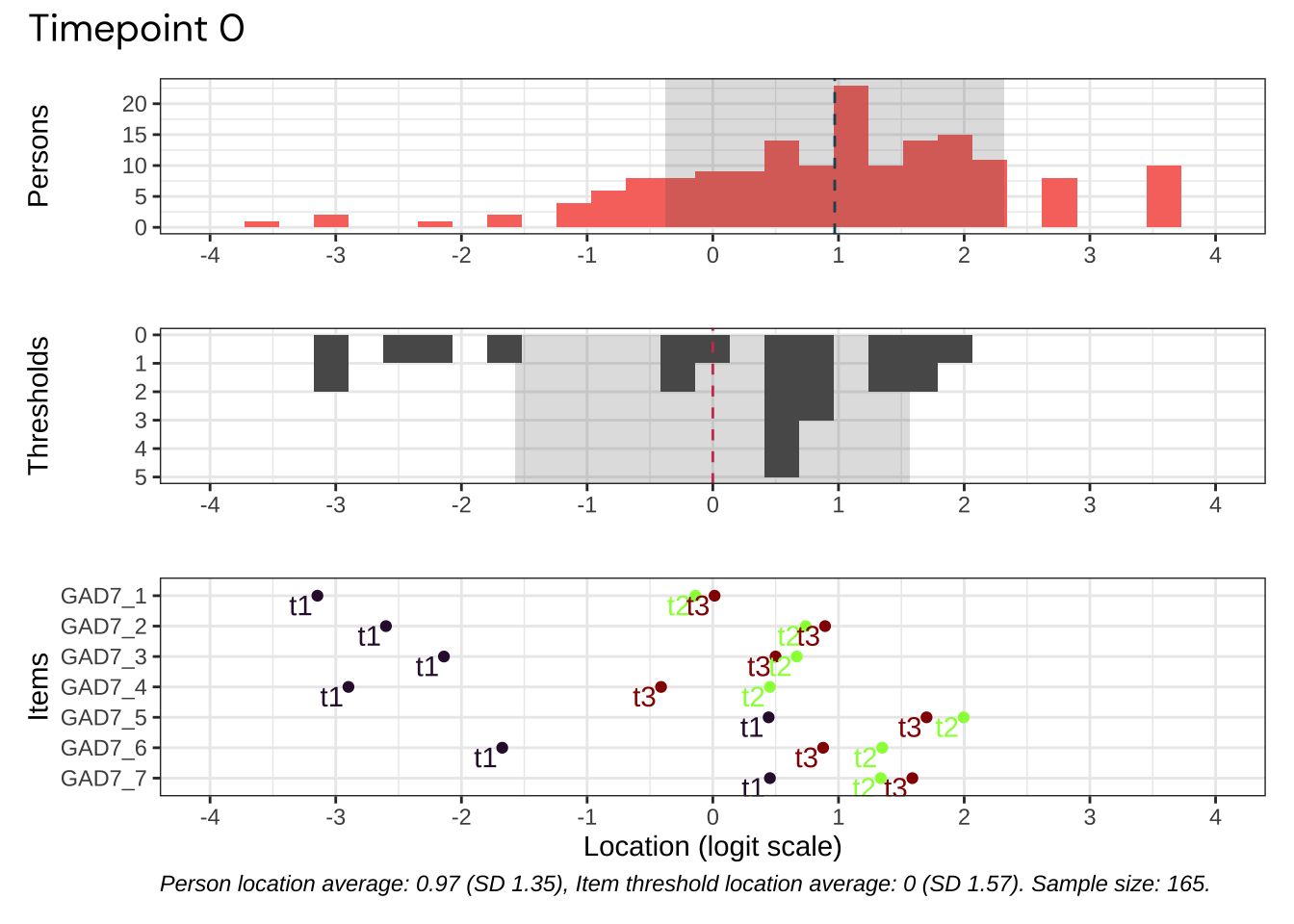
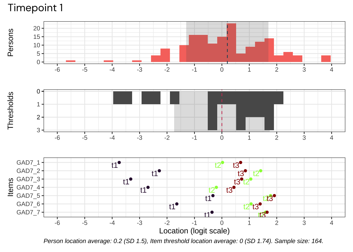
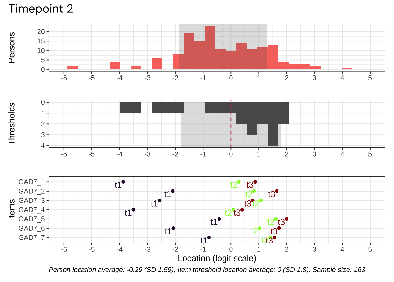
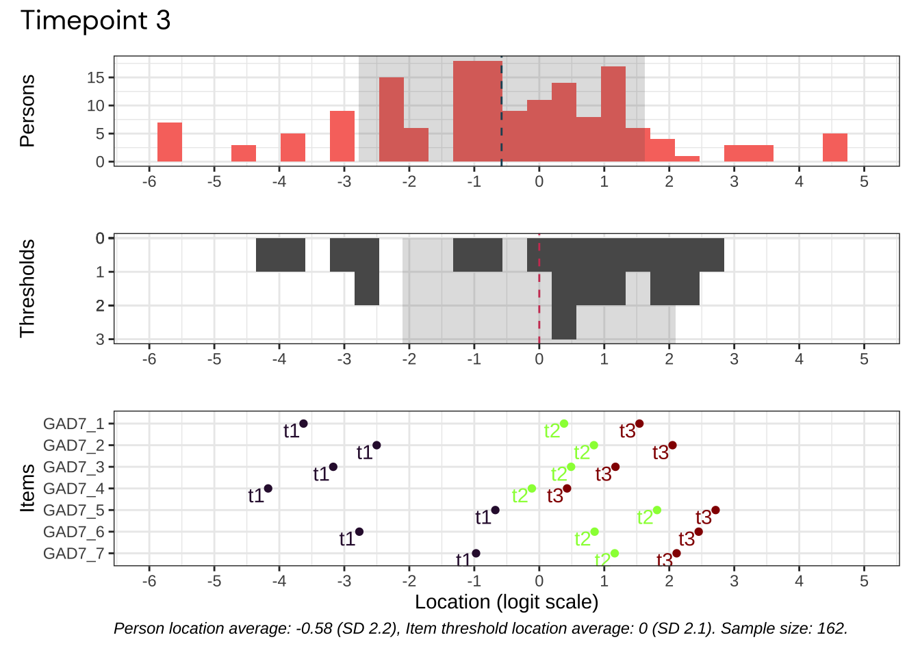
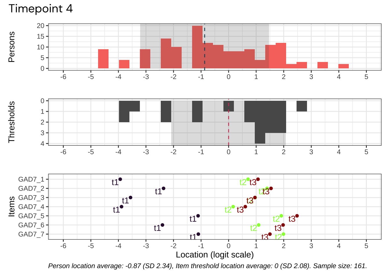
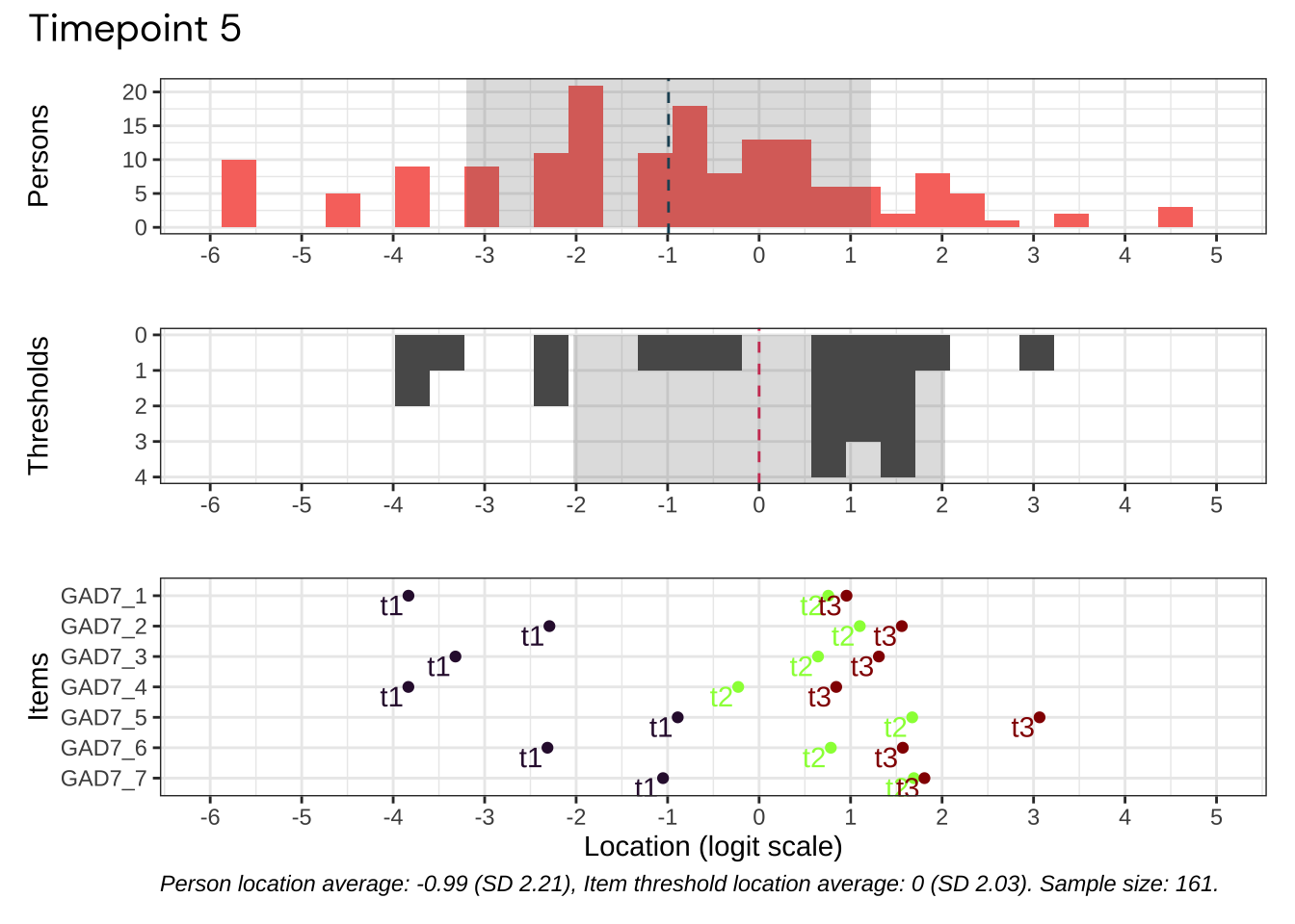
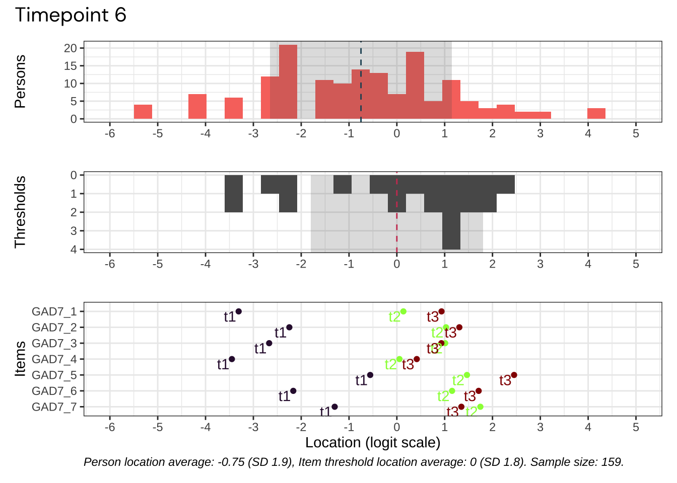
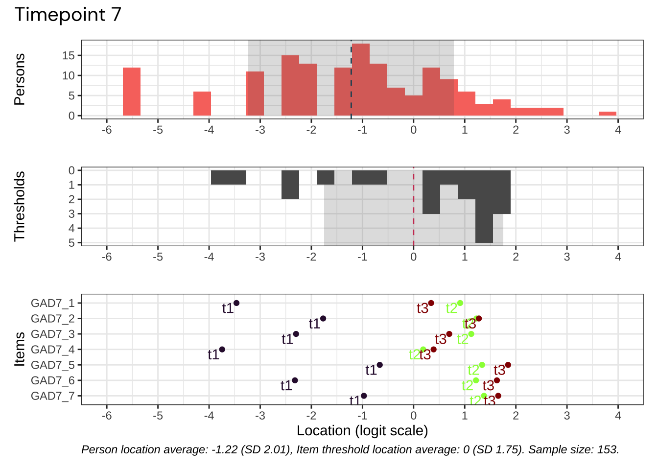
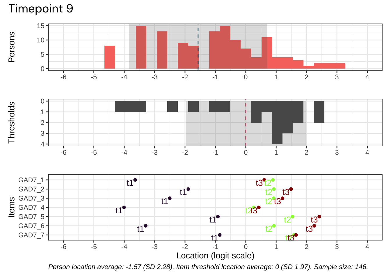
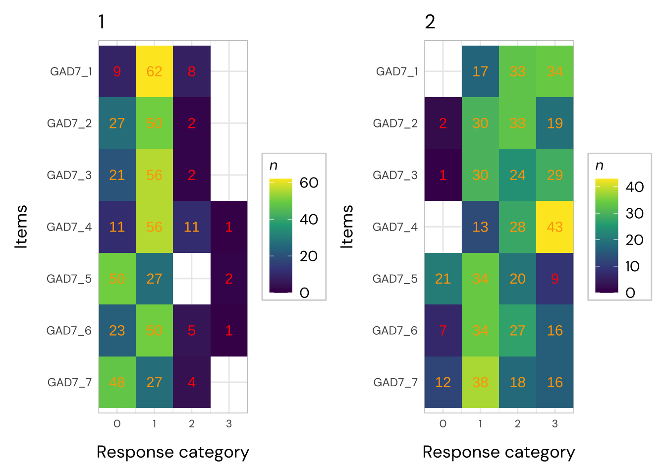
We’ll select the datapoint with best targeting for our psychometric analysis.

Code

plots <- d %>% 
  add_column(time = dif.time) %>% 
  na.omit() %>% 
  split(.$time) %>% 
  map(~ RItargeting(.x %>% select(!time)) + plot_annotation(title = paste0("Timepoint ",.x$time)))

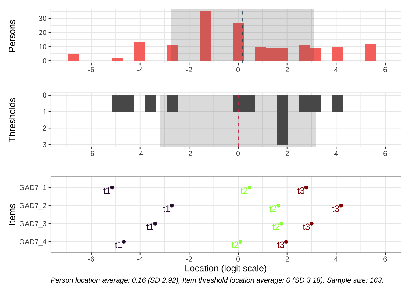
Code

plots[[1]]
plots[[2]]
plots[[3]]
plots[[4]]
plots[[5]]
plots[[6]]
plots[[7]]
plots[[8]]
plots[[9]]
plots[[10]]

Looks like timepoint 2 is best targeted, and has a sample size of 163 complete responses.

Code

d <- d %>% 
  add_column(time = dif.time) %>% 
  filter(time == 2) %>% 
  na.omit() %>% 
  select(!time)

5.1.1 Descriptives

Code

RItileplot(d)

Code

RIbarstack(d)

Code

RIitemcols(d)

5.2 Rasch analysis 1

The eRm package, which uses Conditional Maximum Likelihood (CML) estimation, will be used primarily. For this analysis, the Partial Credit Model will be used.

itemnr	item
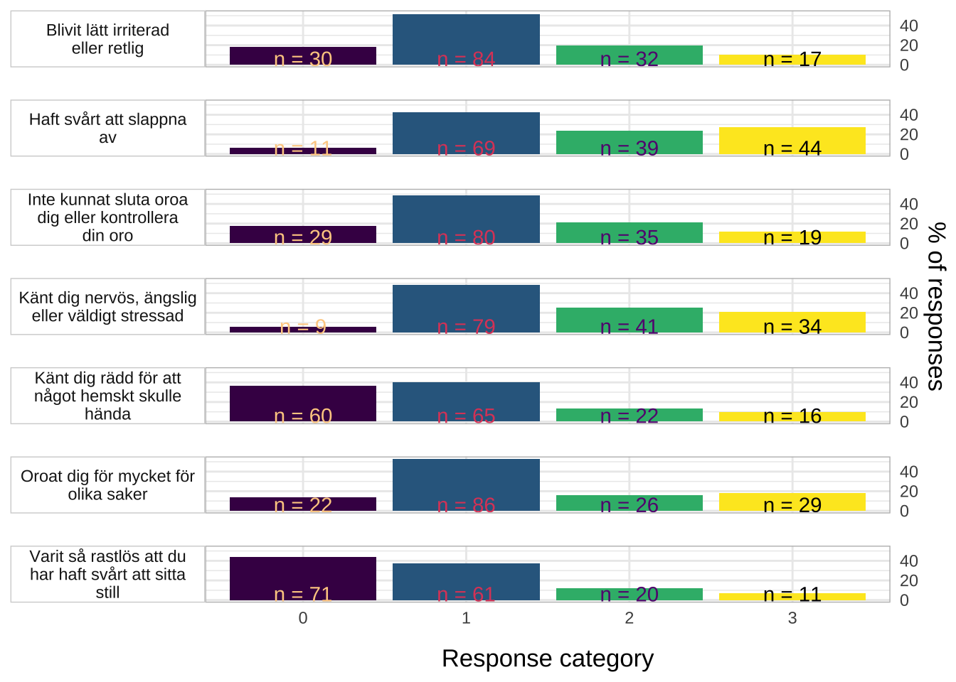
GAD7_1	Känt dig nervös, ängslig eller väldigt stressad
GAD7_2	Inte kunnat sluta oroa dig eller kontrollera din oro
GAD7_3	Oroat dig för mycket för olika saker
GAD7_4	Haft svårt att slappna av
GAD7_5	Varit så rastlös att du har haft svårt att sitta still
GAD7_6	Blivit lätt irriterad eller retlig
GAD7_7	Känt dig rädd för att något hemskt skulle hända

Code

simfit1 <- RIgetfit(d, iterations = 100, cpu = 8) 
RIitemfit(d, simfit1)

Item	InfitMSQ	Infit thresholds	OutfitMSQ	Outfit thresholds	Infit diff	Outfit diff	Relative location
GAD7_1	0.693	[0.735, 1.213]	0.642	[0.704, 1.42]	0.042	0.062	-0.61
GAD7_2	0.601	[0.834, 1.242]	0.584	[0.832, 1.26]	0.233	0.248	0.42
GAD7_3	0.651	[0.791, 1.314]	0.608	[0.758, 1.302]	0.14	0.15	0.06
GAD7_4	0.799	[0.774, 1.256]	0.758	[0.751, 1.359]	no misfit	no misfit	-0.71
GAD7_5	1.576	[0.773, 1.178]	1.94	[0.712, 1.475]	0.398	0.465	1.35
GAD7_6	1.281	[0.752, 1.396]	1.406	[0.74, 1.488]	no misfit	no misfit	0.52
GAD7_7	1.334	[0.811, 1.202]	1.328	[0.772, 1.534]	0.132	no misfit	1.02
Note:
MSQ values based on conditional calculations (n = 163 complete cases). Simulation based thresholds from 100 simulated datasets.

Code

RIrestscore(d)

Item	Observed value	Model expected value	Absolute difference	Adjusted p-value (BH)	Statistical significance level	Location	Relative location
GAD7_1	0.77	0.64	0.13	0.001	***	-0.91	-0.61
GAD7_2	0.81	0.62	0.19	0.000	***	0.12	0.42
GAD7_3	0.81	0.65	0.16	0.000	***	-0.23	0.06
GAD7_4	0.73	0.64	0.09	0.072	.	-1.00	-0.71
GAD7_5	0.42	0.62	0.20	0.020	*	1.06	1.35
GAD7_6	0.51	0.62	0.11	0.098	.	0.23	0.52
GAD7_7	0.51	0.62	0.11	0.096	.	0.73	1.02

Code

RIpcmPCA(d)

PCA of Rasch model residuals
Eigenvalues	Proportion of variance
1.94	30.8%
1.48	23.4%
1.15	21.7%
0.90	10.2%
0.79	7.2%

Code

simcor1 <- RIgetResidCor(d, iterations = 500, cpu = 8)
RIresidcorr(d, cutoff = simcor1$p99)

	GAD7_1	GAD7_2	GAD7_3	GAD7_4	GAD7_5	GAD7_6
GAD7_1
GAD7_2	0.27
GAD7_3	0.14	0.21
GAD7_4	0.16	0.04	-0.11
GAD7_5	-0.36	-0.32	-0.44	-0.07
GAD7_6	-0.26	-0.32	-0.13	-0.23	-0.08
GAD7_7	-0.28	-0.16	-0.06	-0.37	-0.18	-0.18
Note:
Relative cut-off value is 0.144, which is 0.274 above the average correlation (-0.13). Correlations above the cut-off are highlighted in red text.

Code

RIloadLoc(d)

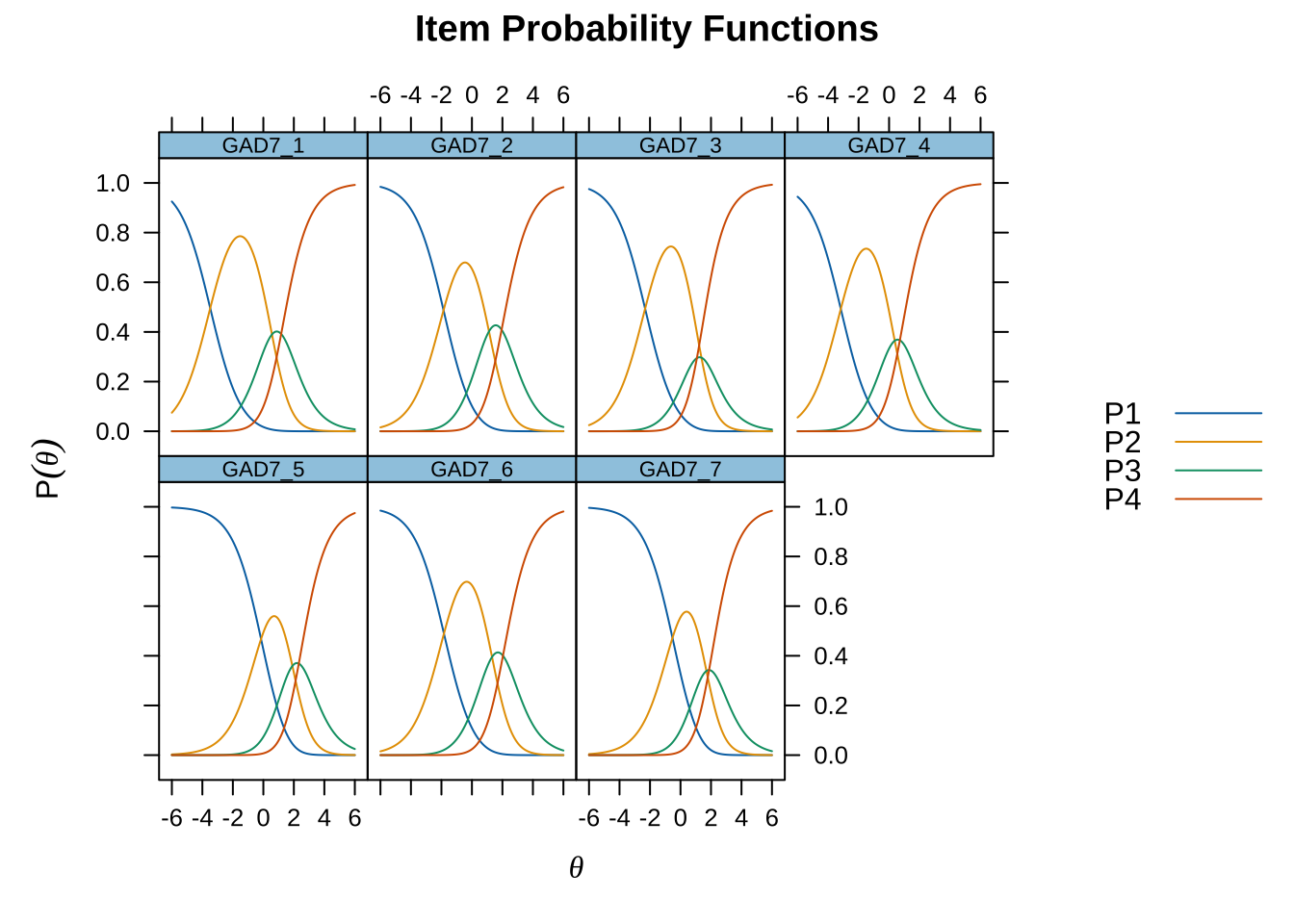
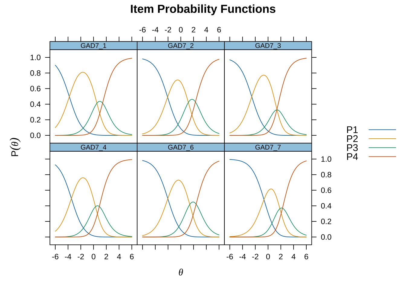
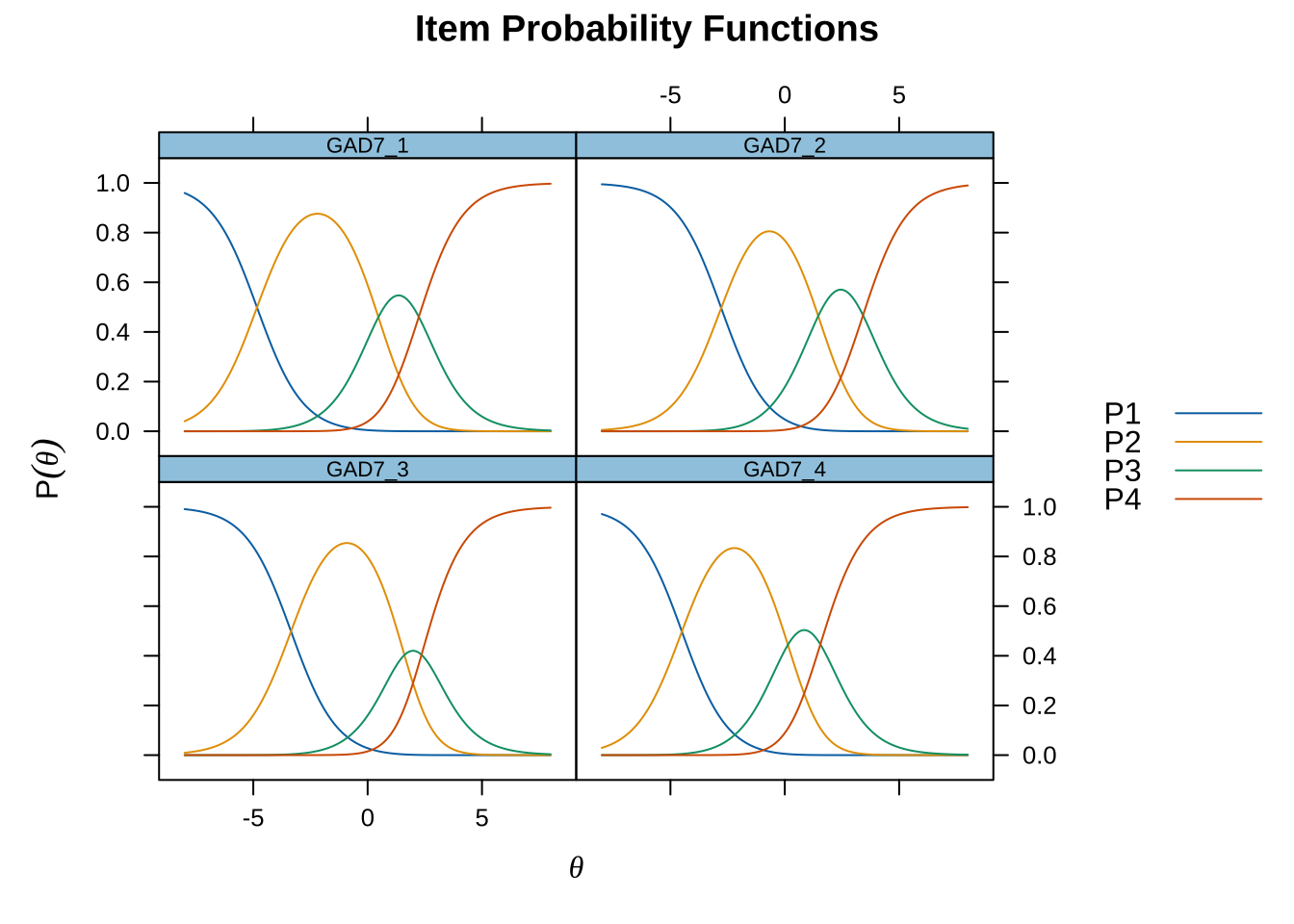
Code

mirt(d, model=1, itemtype='Rasch', verbose = FALSE) %>% 
  plot(type="trace", as.table = TRUE, 
       theta_lim = c(-6,6))

Code

# for fewer items or a more magnified figure, use:
#RIitemCats(df)

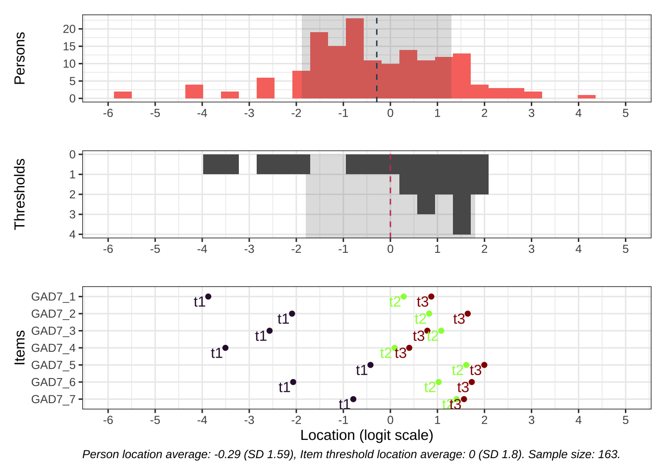
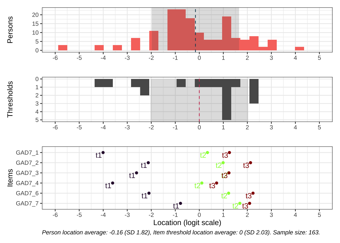
Code

# increase fig-height above as needed, if you have many items
RItargeting(d)

Code

RIitemHierarchy(d)

Code

iarm::score_groups(as.data.frame(d)) %>% 
  as.data.frame(nm = "score_group") %>% 
  dplyr::count(score_group)

  score_group  n
1           1 79
2           2 84

Code

dif_plots <- d %>% 
  add_column(dif = iarm::score_groups(.)) %>% 
  split(.$dif) %>% # split the data using the DIF variable
  map(~ RItileplot(.x %>% dplyr::select(!dif)) + labs(title = .x$dif))
dif_plots[[1]] + dif_plots[[2]]

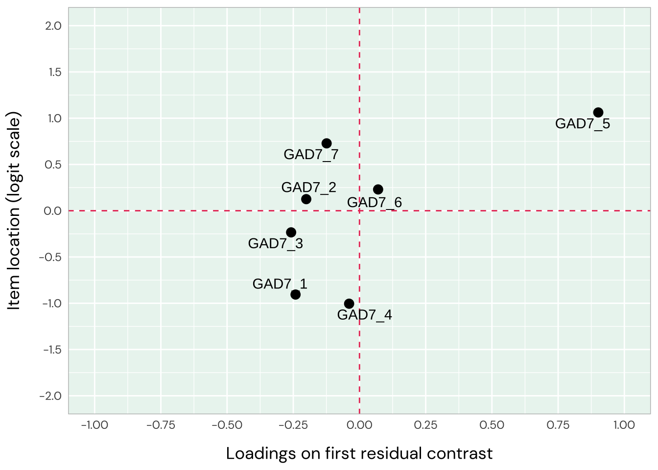
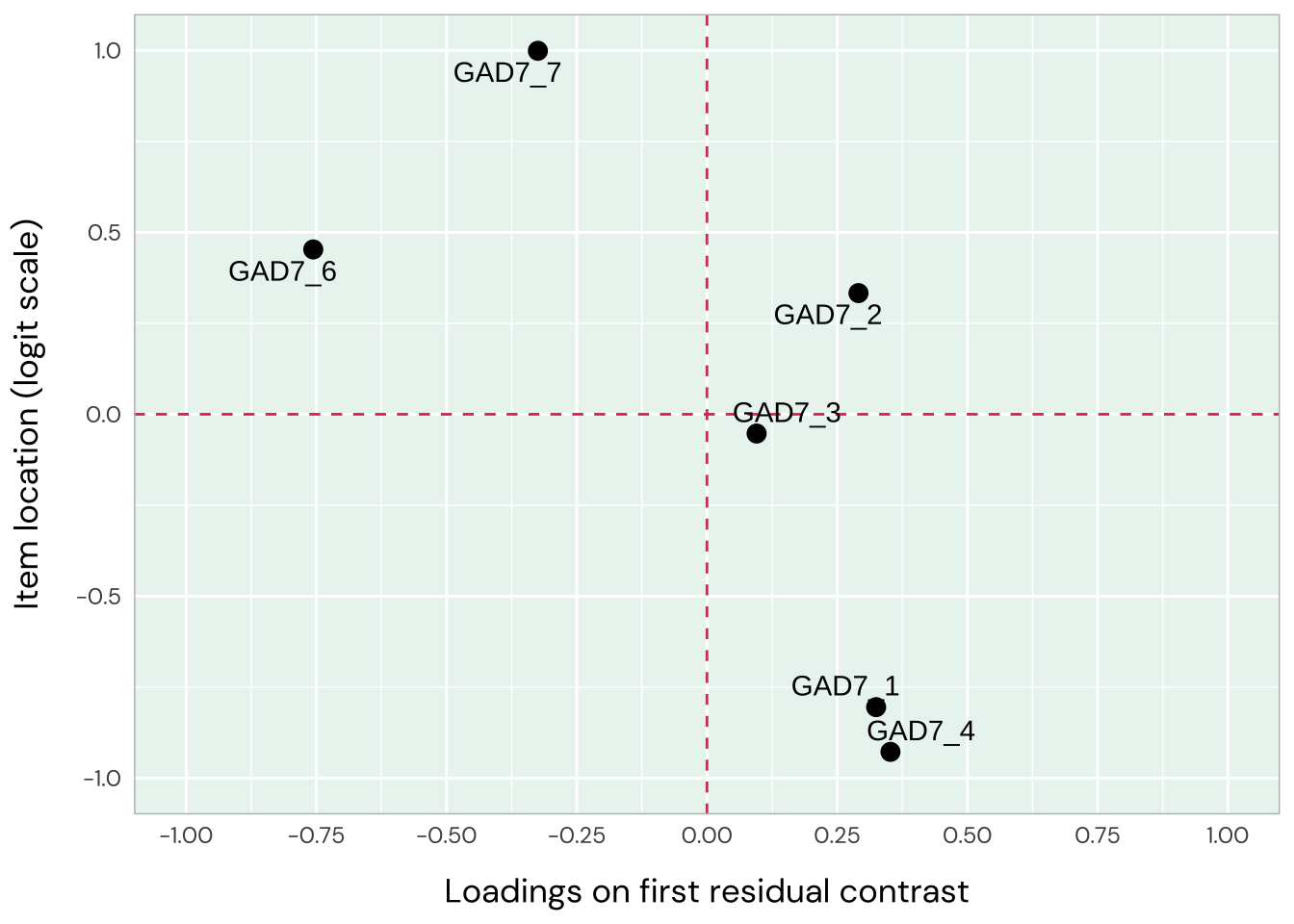
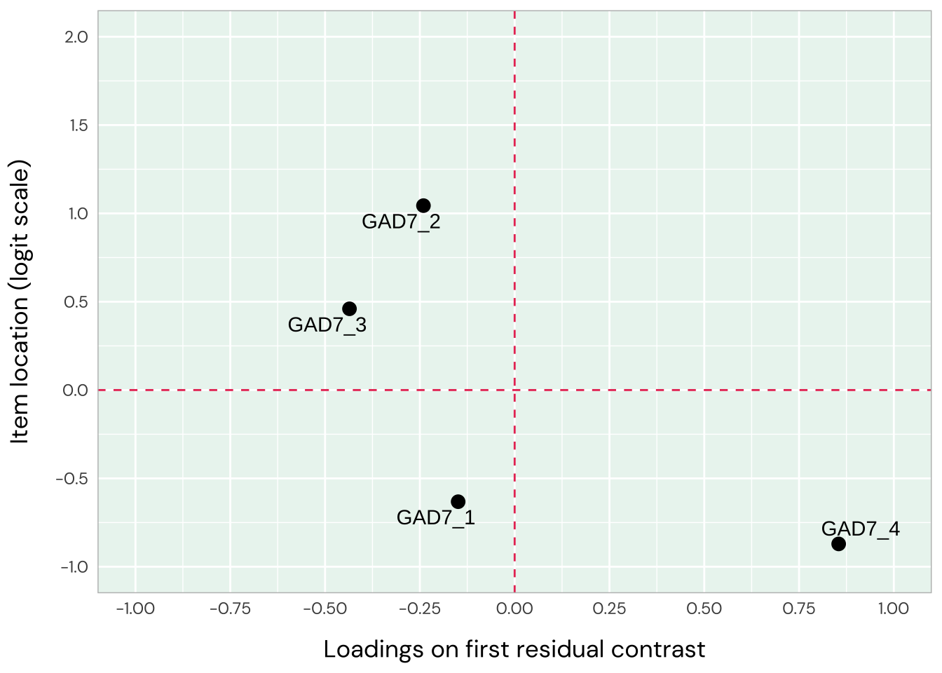
Item 1 has residual correlations with item 2 and 4, while 2 and 3 are also locally dependent. Items 1-3 are all overfit, whileiItems 5-7 are underfit (high item infit, particularly item 5 and to a lesser degree 7). This indicates two dimensions in data. The loadings plot does not show this as clearly, though, with item 5 being the only item deviating strongly.

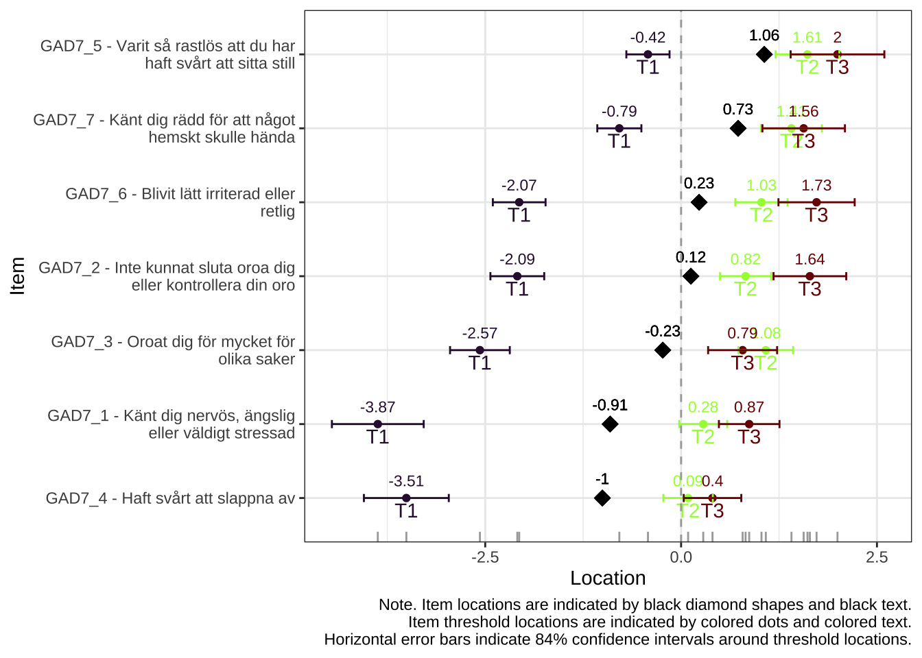
All items have issues with the second highest response category having very small distance from the adjancent item category threshold locations.

The sample is too small to create score groups for DIF analysis based on low/high scores.

5.3 Rasch analysis 2

While two dimensions seems likely, let’s see if we can find a working set of unidimensional items based on all 7. First, we remove item 5, leaving other issues for later.

Code

d.backup <- d

d$GAD7_5 <- NULL

itemnr	item
GAD7_1	Känt dig nervös, ängslig eller väldigt stressad
GAD7_2	Inte kunnat sluta oroa dig eller kontrollera din oro
GAD7_3	Oroat dig för mycket för olika saker
GAD7_4	Haft svårt att slappna av
GAD7_6	Blivit lätt irriterad eller retlig
GAD7_7	Känt dig rädd för att något hemskt skulle hända

Code

simfit1 <- RIgetfit(d, iterations = 100, cpu = 8) 

RIitemfit(d, simfit1)

Item	InfitMSQ	Infit thresholds	OutfitMSQ	Outfit thresholds	Infit diff	Outfit diff	Relative location
GAD7_1	0.718	[0.73, 1.312]	0.68	[0.732, 1.417]	0.012	0.052	-0.64
GAD7_2	0.612	[0.752, 1.275]	0.606	[0.741, 1.314]	0.14	0.135	0.50
GAD7_3	0.631	[0.74, 1.304]	0.574	[0.713, 1.365]	0.109	0.139	0.11
GAD7_4	0.975	[0.793, 1.256]	1.012	[0.725, 1.243]	no misfit	no misfit	-0.76
GAD7_6	1.501	[0.793, 1.22]	1.633	[0.764, 1.369]	0.281	0.264	0.62
GAD7_7	1.514	[0.738, 1.32]	1.452	[0.694, 1.628]	0.194	no misfit	1.16
Note:
MSQ values based on conditional calculations (n = 163 complete cases). Simulation based thresholds from 100 simulated datasets.

Code

RIrestscore(d)

Item	Observed value	Model expected value	Absolute difference	Adjusted p-value (BH)	Statistical significance level	Location	Relative location
GAD7_1	0.81	0.69	0.12	0.001	***	-0.80	-0.64
GAD7_2	0.82	0.67	0.15	0.000	***	0.33	0.50
GAD7_3	0.85	0.70	0.15	0.000	***	-0.05	0.11
GAD7_4	0.71	0.69	0.02	0.721		-0.93	-0.76
GAD7_6	0.49	0.67	0.18	0.022	*	0.45	0.62
GAD7_7	0.52	0.66	0.14	0.037	*	1.00	1.16

Code

RIpcmPCA(d)

PCA of Rasch model residuals
Eigenvalues	Proportion of variance
1.81	33.7%
1.36	30.8%
1.10	16.1%
0.88	10.1%
0.84	9.1%

Code

simcor1 <- RIgetResidCor(d, iterations = 500, cpu = 8)
RIresidcorr(d, cutoff = simcor1$p99)

	GAD7_1	GAD7_2	GAD7_3	GAD7_4	GAD7_6
GAD7_1
GAD7_2	0.18
GAD7_3	-0.01	0.08
GAD7_4	0.1	-0.01	-0.21
GAD7_6	-0.33	-0.39	-0.2	-0.23
GAD7_7	-0.37	-0.25	-0.15	-0.4	-0.19
Note:
Relative cut-off value is 0.115, which is 0.274 above the average correlation (-0.158). Correlations above the cut-off are highlighted in red text.

Code

RIloadLoc(d)

Code

mirt(d, model=1, itemtype='Rasch', verbose = FALSE) %>% 
  plot(type="trace", as.table = TRUE, 
       theta_lim = c(-6,6))

Code

# increase fig-height above as needed, if you have many items
RItargeting(d)

Code

RIitemHierarchy(d)

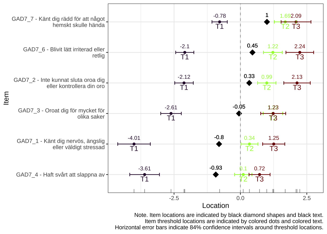
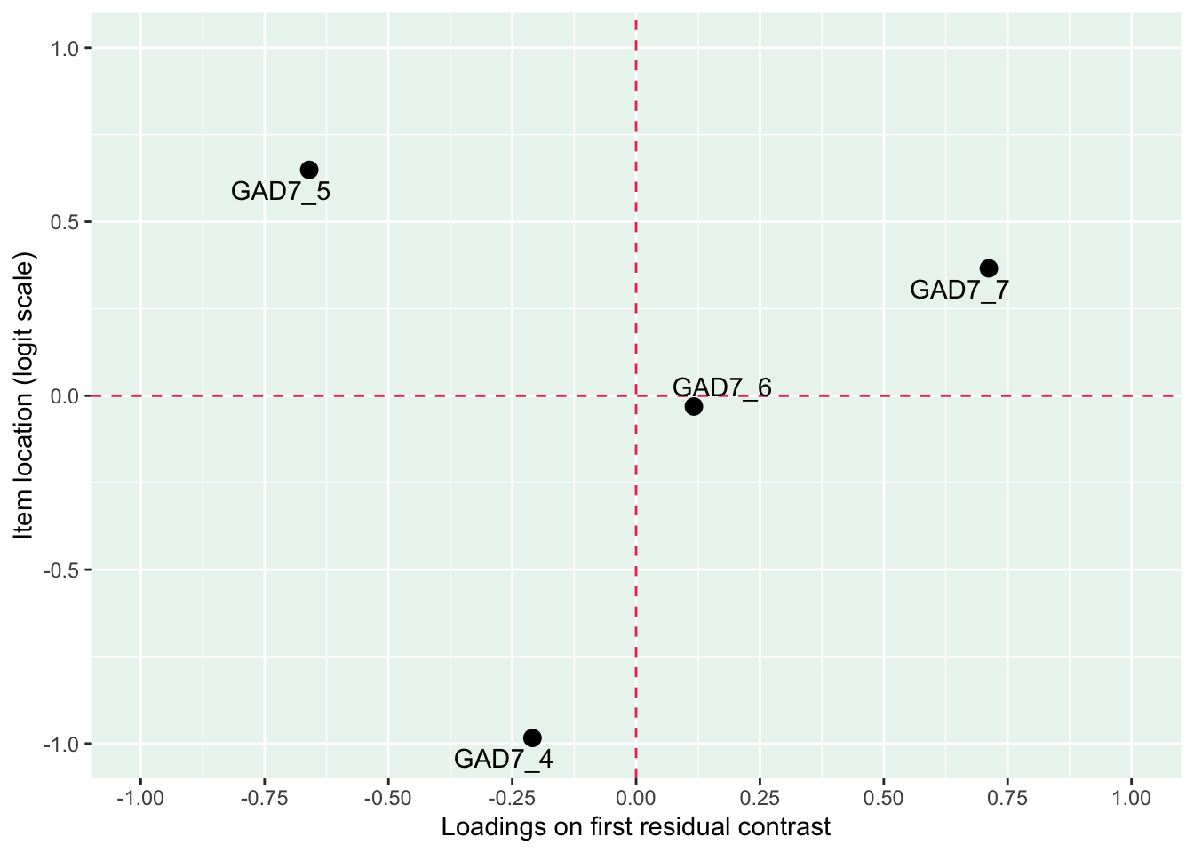
Only items 1 and 2 have a residual correlation now. The pattern in underfit and overfit items is more clearly seen in the loadings/location plot, with items 6 and 7 deviating. This confirms the two-dimensional structure, and we’ll move to look at items 1-4 and 4-7 separately.

5.4 Two separate dimensions

The initial analysis with all 7 items indicated that items 1-3 have low item fit (overfit to the Rasch model) strong residual correlations amongst them. This could mean that these items work well together, but likely represent another dimension than items 5-7, which in turn all showed high item fit (underfit).

We’ll make an analysis of this setup, including item 4 with both sets.

Code

d1 <- d[,1:4]
d2 <- d.backup[,4:7]

5.5 Items 1-4, worry

Code

d <- d1

itemnr	item
GAD7_1	Känt dig nervös, ängslig eller väldigt stressad
GAD7_2	Inte kunnat sluta oroa dig eller kontrollera din oro
GAD7_3	Oroat dig för mycket för olika saker
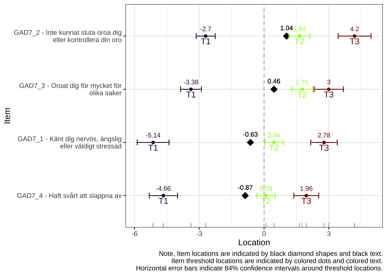
GAD7_4	Haft svårt att slappna av

Code

simfit1 <- RIgetfit(d, iterations = 100, cpu = 8) 

RIitemfit(d, simfit1)

Item	InfitMSQ	Infit thresholds	OutfitMSQ	Outfit thresholds	Infit diff	Outfit diff	Relative location
GAD7_1	0.845	[0.755, 1.251]	0.725	[0.696, 1.523]	no misfit	no misfit	-0.79
GAD7_2	0.781	[0.845, 1.25]	0.739	[0.742, 1.381]	0.064	0.003	0.88
GAD7_3	1.107	[0.686, 1.298]	0.891	[0.618, 1.735]	no misfit	no misfit	0.30
GAD7_4	1.264	[0.779, 1.255]	1.314	[0.609, 1.36]	0.009	no misfit	-1.03
Note:
MSQ values based on conditional calculations (n = 163 complete cases). Simulation based thresholds from 100 simulated datasets.

Code

RIrestscore(d)

Item	Observed value	Model expected value	Absolute difference	Adjusted p-value (BH)	Location	Relative location
GAD7_1	0.88	0.83	0.05	0.177	-0.63	-0.79
GAD7_2	0.88	0.83	0.05	0.214	1.04	0.88
GAD7_3	0.84	0.85	0.01	0.824	0.46	0.30
GAD7_4	0.79	0.82	0.03	0.577	-0.87	-1.03

Code

simpca <- RIbootPCA(d,200, cpu = 8)
simpca$max

[1] 1.745

Code

RIpcmPCA(d)

PCA of Rasch model residuals
Eigenvalues	Proportion of variance
1.49	44.8%
1.29	29.7%
1.20	25.1%
0.02	0.4%

Code

simcor1 <- RIgetResidCor(d, iterations = 500, cpu = 8)
RIresidcorr(d, cutoff = simcor1$p99)

	GAD7_1	GAD7_2	GAD7_3
GAD7_1
GAD7_2	-0.14
GAD7_3	-0.27	-0.14
GAD7_4	-0.24	-0.33	-0.45
Note:
Relative cut-off value is -0.031, which is 0.231 above the average correlation (-0.262). Correlations above the cut-off are highlighted in red text.

Code

RIloadLoc(d)

Code

mirt(d, model=1, itemtype='Rasch', verbose = FALSE) %>% 
  plot(type="trace", as.table = TRUE, 
       theta_lim = c(-8,8))

Code

# increase fig-height above as needed, if you have many items
RItargeting(d)

Code

RIitemHierarchy(d)

Item-restscore looks good. Item infit shows slight overfit item 2. No residual correlations.

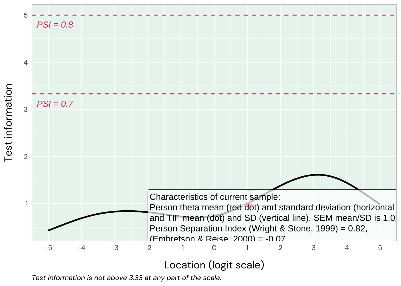
5.5.1 Reliability

Code

RItif(d, samplePSI = T)

TIF is low while PSI is ok at 0.82.

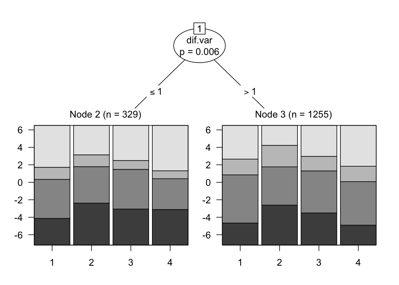
5.5.2 DIF

Code

d <- d.all %>% 
  select(GAD7_1:GAD7_4,time) %>% 
  na.omit()

dif.time <- d$time
d$time <- NULL
RIpartgamDIF(d,dif.time)

[1] "No statistically significant DIF found."

Code

RIdifTable(d,dif.time)

Item	2	3	Mean location	StDev	MaxDiff
GAD7_1	-0.693	-0.388	-0.540	0.216	0.306
GAD7_2	0.851	1.129	0.990	0.196	0.278
GAD7_3	0.304	0.256	0.280	0.034	0.048
GAD7_4	-0.461	-0.997	-0.729	0.379	0.536

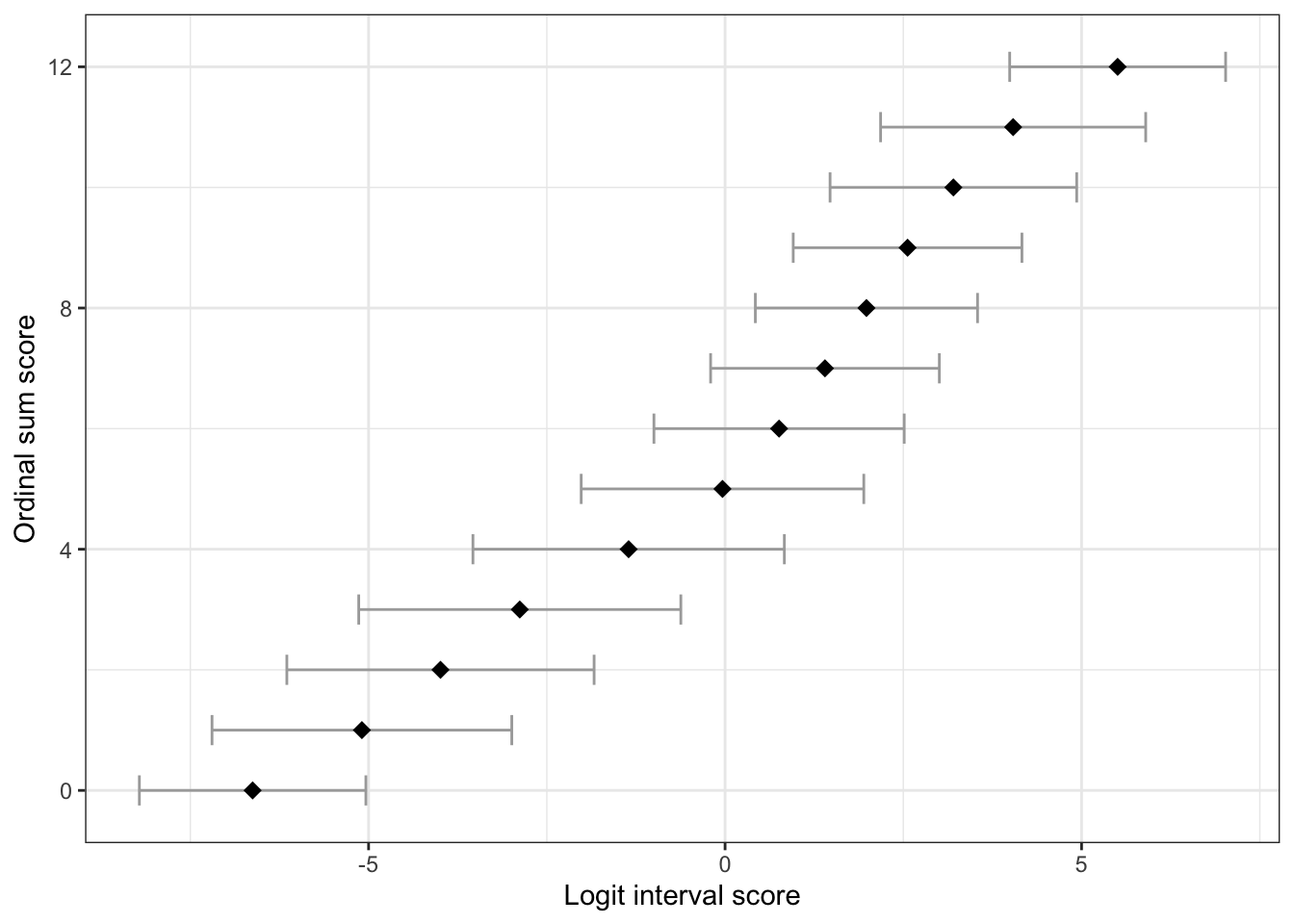
5.5.3 Item parameters

Code

RIitemparams(d1, output = "file", filename = "GAD4_itemparams.csv")
RIscoreSE(d1)

Ordinal sum score	Logit score	Logit std.error
0	-6.626	0.810
1	-5.094	1.073
2	-3.992	1.099
3	-2.879	1.152
4	-1.353	1.114
5	-0.036	1.011
6	0.757	0.896
7	1.401	0.818
8	1.983	0.795
9	2.560	0.818
10	3.202	0.882
11	4.040	0.948
12	5.506	0.773

Code

RIscoreSE(d1, output = "figure")

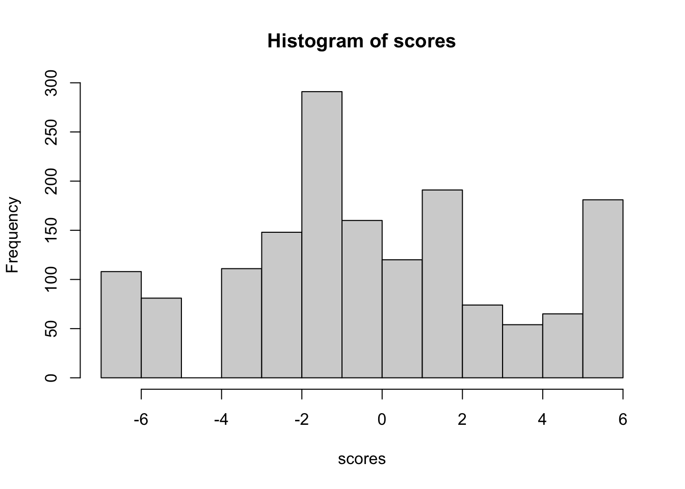
5.5.4 Latent scores items 1-4

Code

itemps <- read_csv("GAD4_itemparams.csv") %>% 
  as.matrix()

d <- df %>% 
  select(GAD7_1:GAD7_4,PID,time) %>% 
  na.omit()

PID <- d$PID
dif.time <- d$time

d <- d %>% 
  select(!c(PID,time))

scores <- RIestThetasCATr(d, itemps, theta_range = c(-8,8))
hist(scores)

Code

summary(scores)

   Min. 1st Qu.  Median    Mean 3rd Qu.    Max. 
-6.6262 -2.8791 -0.0363 -0.2278  1.9828  5.5062

Code

data.frame(PID = PID,
           time = dif.time,
           GAD4_score = scores) %>% 
  write_csv("GAD4_score.csv")

5.6 Items 4-7, anxiety

Code

d <- d2

itemnr	item
GAD7_4	Haft svårt att slappna av
GAD7_5	Varit så rastlös att du har haft svårt att sitta still
GAD7_6	Blivit lätt irriterad eller retlig
GAD7_7	Känt dig rädd för att något hemskt skulle hända

Code

simfit1 <- RIgetfit(d, iterations = 100, cpu = 8) 
RIitemfit(d, simfit1)

Item	InfitMSQ	Infit thresholds	OutfitMSQ	Outfit thresholds	Infit diff	Outfit diff	Relative location
GAD7_4	0.816	[0.833, 1.206]	0.788	[0.797, 1.382]	0.017	0.009	-0.59
GAD7_5	1.054	[0.817, 1.245]	1.034	[0.76, 1.487]	no misfit	no misfit	1.04
GAD7_6	0.982	[0.803, 1.166]	0.995	[0.819, 1.214]	no misfit	no misfit	0.36
GAD7_7	1.148	[0.793, 1.265]	1.055	[0.788, 1.253]	no misfit	no misfit	0.76
Note:
MSQ values based on conditional calculations (n = 163 complete cases). Simulation based thresholds from 100 simulated datasets.

Code

RIrestscore(d)

Item	Observed value	Model expected value	Absolute difference	Adjusted p-value (BH)	Location	Relative location
GAD7_4	0.57	0.47	0.10	0.366	-0.98	-0.59
GAD7_5	0.43	0.46	0.03	0.760	0.65	1.04
GAD7_6	0.49	0.46	0.03	0.760	-0.03	0.36
GAD7_7	0.42	0.47	0.05	0.760	0.37	0.76

Code

simpca <- RIbootPCA(d,200, cpu = 8)
simpca$max

[1] 1.735

Code

RIpcmPCA(d)

PCA of Rasch model residuals
Eigenvalues	Proportion of variance
1.45	37.7%
1.32	34.4%
1.23	27.6%
0.01	0.3%

Code

simcor1 <- RIgetResidCor(d, iterations = 500, cpu = 8)
RIresidcorr(d, cutoff = simcor1$p99)

	GAD7_4	GAD7_5	GAD7_6
GAD7_4
GAD7_5	-0.11
GAD7_6	-0.15	-0.24
GAD7_7	-0.24	-0.34	-0.22
Note:
Relative cut-off value is 0.017, which is 0.234 above the average correlation (-0.217). Correlations above the cut-off are highlighted in red text.

Code

RIloadLoc(d)

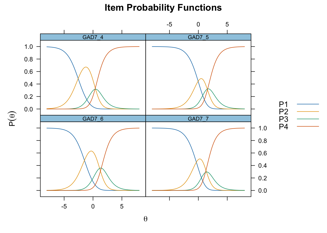
Code

mirt(d, model=1, itemtype='Rasch', verbose = FALSE) %>% 
  plot(type="trace", as.table = TRUE, 
       theta_lim = c(-8,8))

Code

# increase fig-height above as needed, if you have many items
RItargeting(d)

Code

RIitemHierarchy(d)

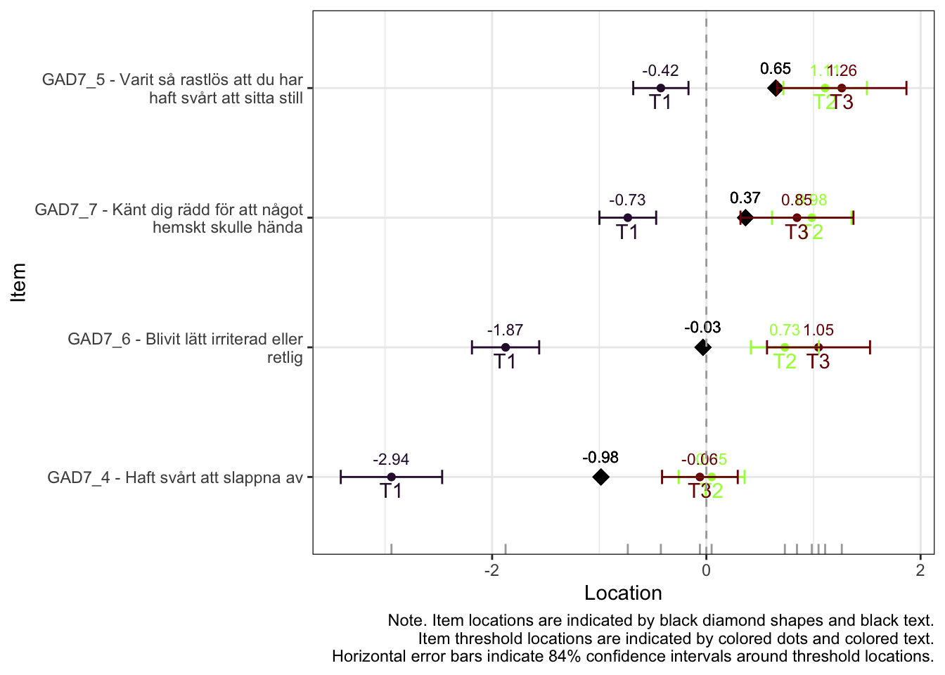
Item 4 actually works quite well with items 5-7 too. However, it shows disordered thresholds in this item set, which it does not with items 1-3, so we will use it as a part of item set 1, “worry”.

Item thresholds have small distances or are disordered (2 items) in this item set, which is further indicated by the low reliability, even before merging response categories. We will not use this second set of items in any analysis.