3 PCS-4 – Return to work questionnaires

Code

library(tidyverse)
library(janitor)
library(skimr)
library(easyRasch)
library(haven)

### some commands exist in multiple packages, here we define preferred ones that are frequently used
select <- dplyr::select
count <- dplyr::count
recode <- car::recode
rename <- dplyr::rename

d.all <- read_spss("data/SUVRTW_LONG 240528 TOTAL.sav") 

d <- d.all %>% 
  select(starts_with("PCS"),time)

# subset and remove DIF variable(s)
dif.time <- d$time
d$time <- NULL

itemlabels <- read_csv("data/spss_labels.csv") %>% 
  filter(str_detect(itemnr,"PCS"))

3.1 Background

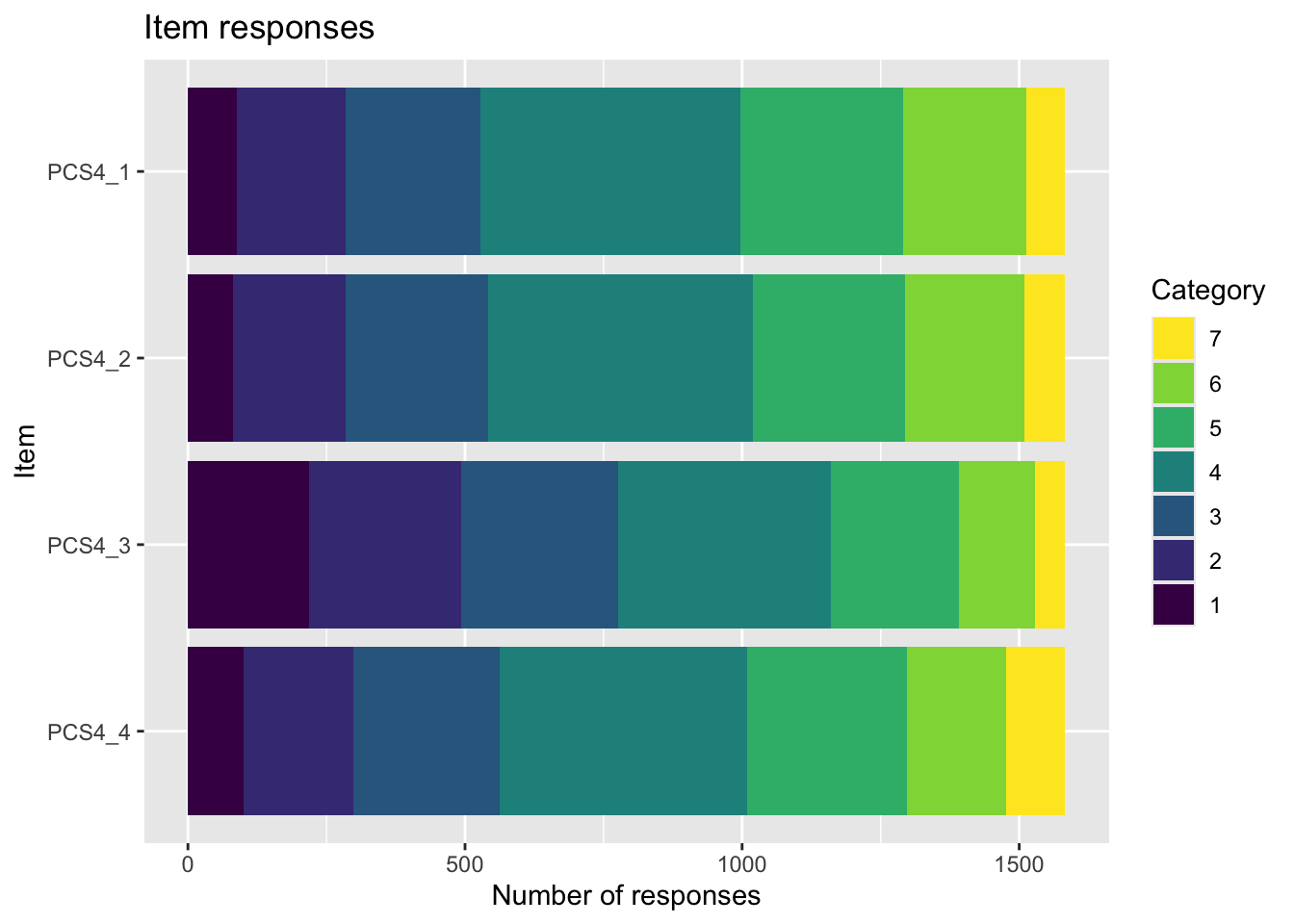
Since these items have 7 response categories we will use a stacked dataset to make sure we have enough responses in each response category.

3.1.1 Descriptives

Code

RItileplot(d)

Code

RIbarstack(d)

Code

RImissing(d)

Code

# n persons w missing
n_complete <- d %>% 
  na.omit() %>% 
  nrow()

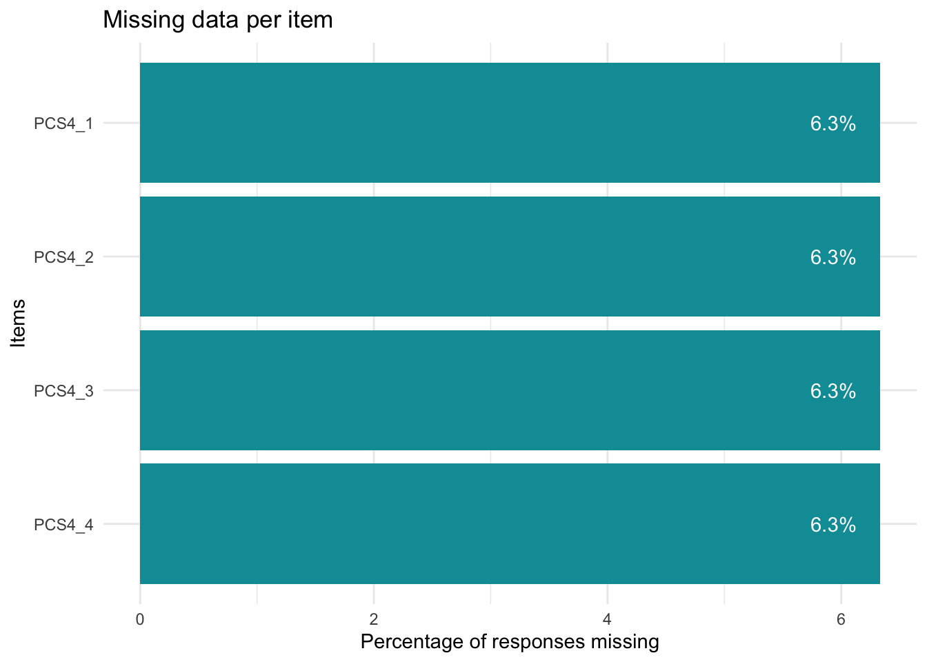
0.9366864 of respondents have complete data (n = 1583). We will remove those with missing data

Code

d <- d.all %>% 
  select(starts_with("PCS"),time,PID) %>% 
  na.omit()

# subset and remove DIF variable(s)
dif.time <- d$time
d$time <- NULL

# subset and remove ID variable
PID <- d$PID
d$PID <- NULL

Code

RItileplot(d)

Code

RIbarstack(d)

Code

RIitemcols(d)

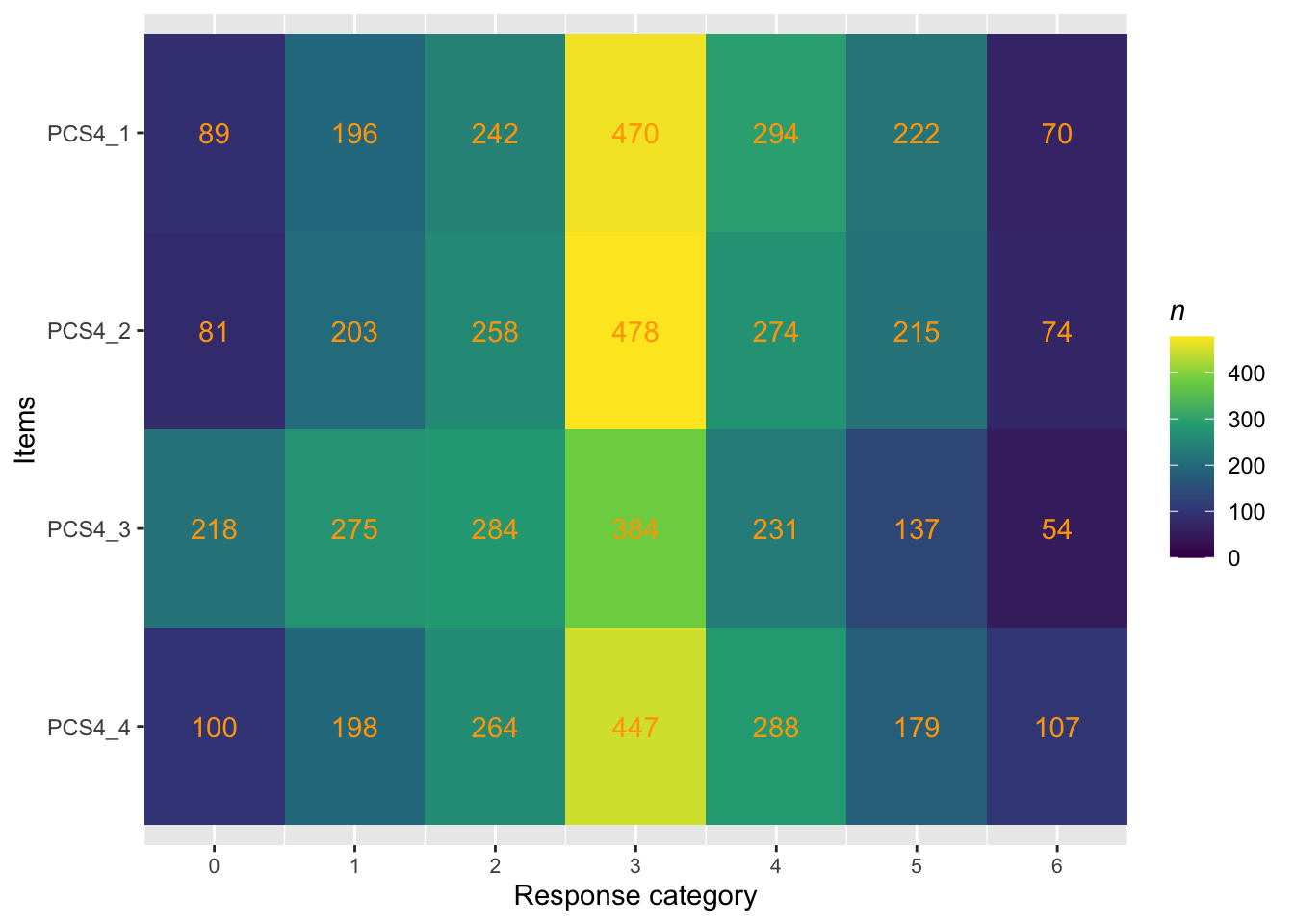
We need to recode to make 0 the lowest response category.

Code

d <- d %>% 
  mutate(across(everything(), ~ .x - 1))
RItileplot(d)

3.2 Rasch analysis 1

The eRm package, which uses Conditional Maximum Likelihood (CML) estimation, will be used primarily. For this analysis, the Partial Credit Model will be used.

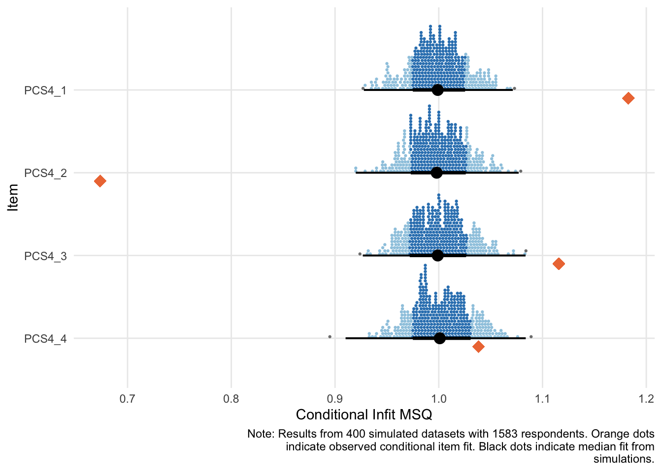
Since we have a large sample size (n > 1000), we’ll add bootstrapped item-restscore as a method for assessing item fit (Johansson, 2025).

itemnr	item
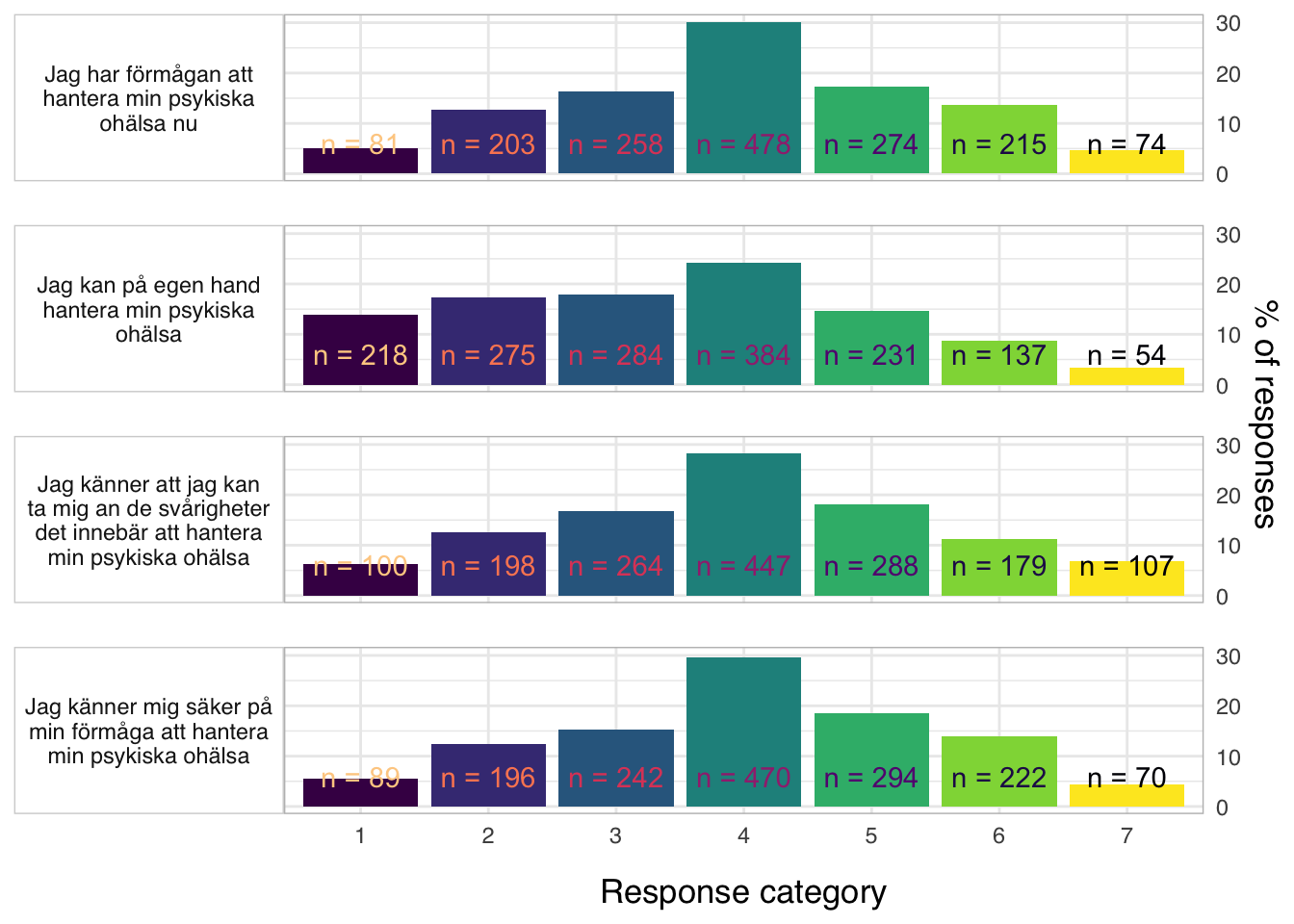
PCS4_1	Jag känner mig säker på min förmåga att hantera min psykiska ohälsa
PCS4_2	Jag har förmågan att hantera min psykiska ohälsa nu
PCS4_3	Jag kan på egen hand hantera min psykiska ohälsa
PCS4_4	Jag känner att jag kan ta mig an de svårigheter det innebär att hantera min psykiska ohälsa

Code

simfit1 <- RIgetfit(d, iterations = 400, cpu = 8) 

RIitemfit(d, simfit1)

Item	InfitMSQ	Infit thresholds	OutfitMSQ	Outfit thresholds	Infit diff	Outfit diff	Relative location
PCS4_1	1.183	[0.928, 1.071]	1.163	[0.92, 1.078]	0.112	0.085	0.11
PCS4_2	0.674	[0.92, 1.077]	0.674	[0.922, 1.086]	0.246	0.248	0.08
PCS4_3	1.116	[0.927, 1.084]	1.114	[0.913, 1.107]	0.032	0.007	0.95
PCS4_4	1.038	[0.91, 1.084]	1.022	[0.908, 1.086]	no misfit	no misfit	0.02
Note:
MSQ values based on conditional calculations (n = 1583 complete cases). Simulation based thresholds from 400 simulated datasets.

Code

RIgetfitPlot(simfit1, d)

Code

RIrestscore(d)

Item	Observed value	Model expected value	Absolute difference	Adjusted p-value (BH)	Statistical significance level	Location	Relative location
PCS4_1	0.74	0.75	0.01	0.891		-0.18	0.11
PCS4_2	0.85	0.75	0.10	0.000	***	-0.21	0.08
PCS4_3	0.73	0.75	0.02	0.540		0.66	0.95
PCS4_4	0.77	0.75	0.02	0.255		-0.27	0.02

Code

RIbootRestscore(d, samplesize = 600, cpu = 8, iterations = 250)

Item	Item-restscore result	% of iterations	Conditional MSQ infit	Relative average item location
PCS4_2	overfit	100.0	0.67	0.08
PCS4_4	overfit	6.4	1.04	0.02
Note:
Results based on 250 bootstrap iterations with n = 600 and 4 items. Conditional mean-square infit based on complete responders only (n = 1583).

Code

RIpcmPCA(d)

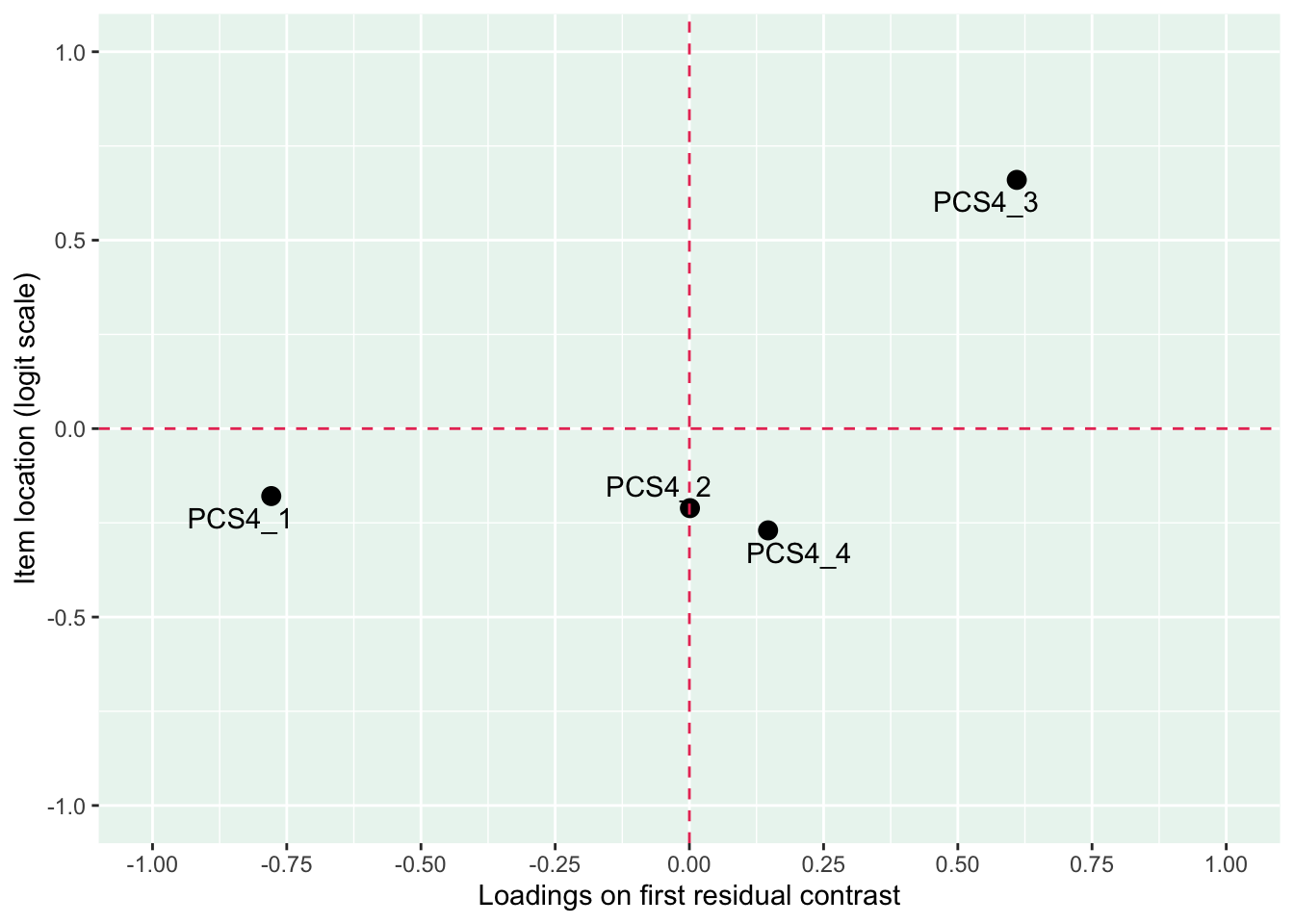
PCA of Rasch model residuals
Eigenvalues	Proportion of variance
1.47	42.2%
1.34	35.2%
1.18	22.5%
0.00	0.1%

Code

simcor <- RIgetResidCor(d,500,8)
RIresidcorr(d, simcor$p99)

	PCS4_1	PCS4_2	PCS4_3
PCS4_1
PCS4_2	-0.2
PCS4_3	-0.44	-0.2
PCS4_4	-0.36	-0.22	-0.35
Note:
Relative cut-off value is -0.22, which is 0.075 above the average correlation (-0.295). Correlations above the cut-off are highlighted in red text.

Code

RIloadLoc(d)

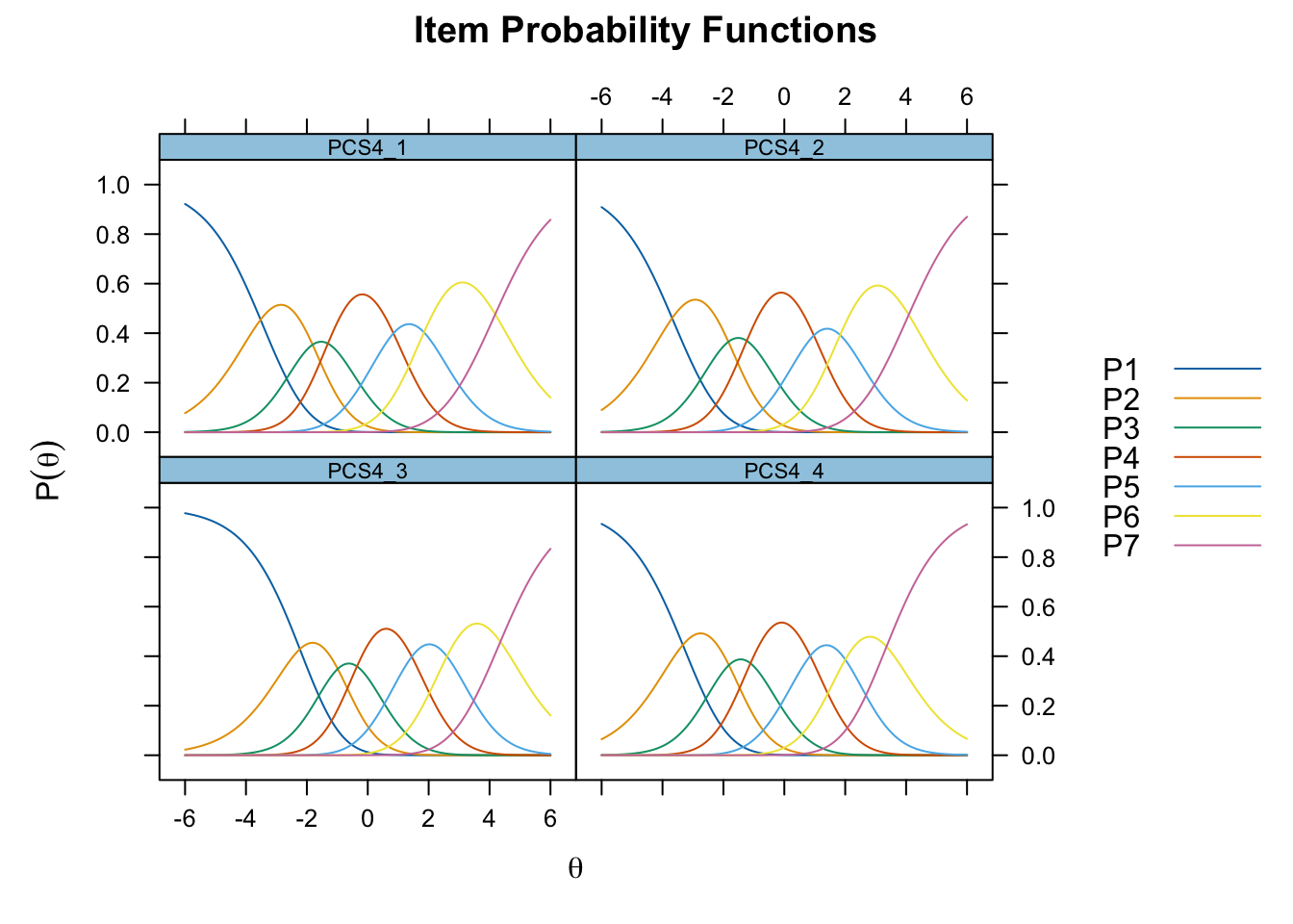
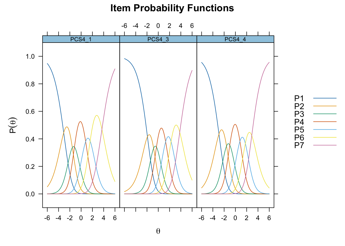
Code

mirt(d, model=1, itemtype='Rasch', verbose = FALSE) %>% 
  plot(type="trace", as.table = TRUE, 
       theta_lim = c(-6,6))

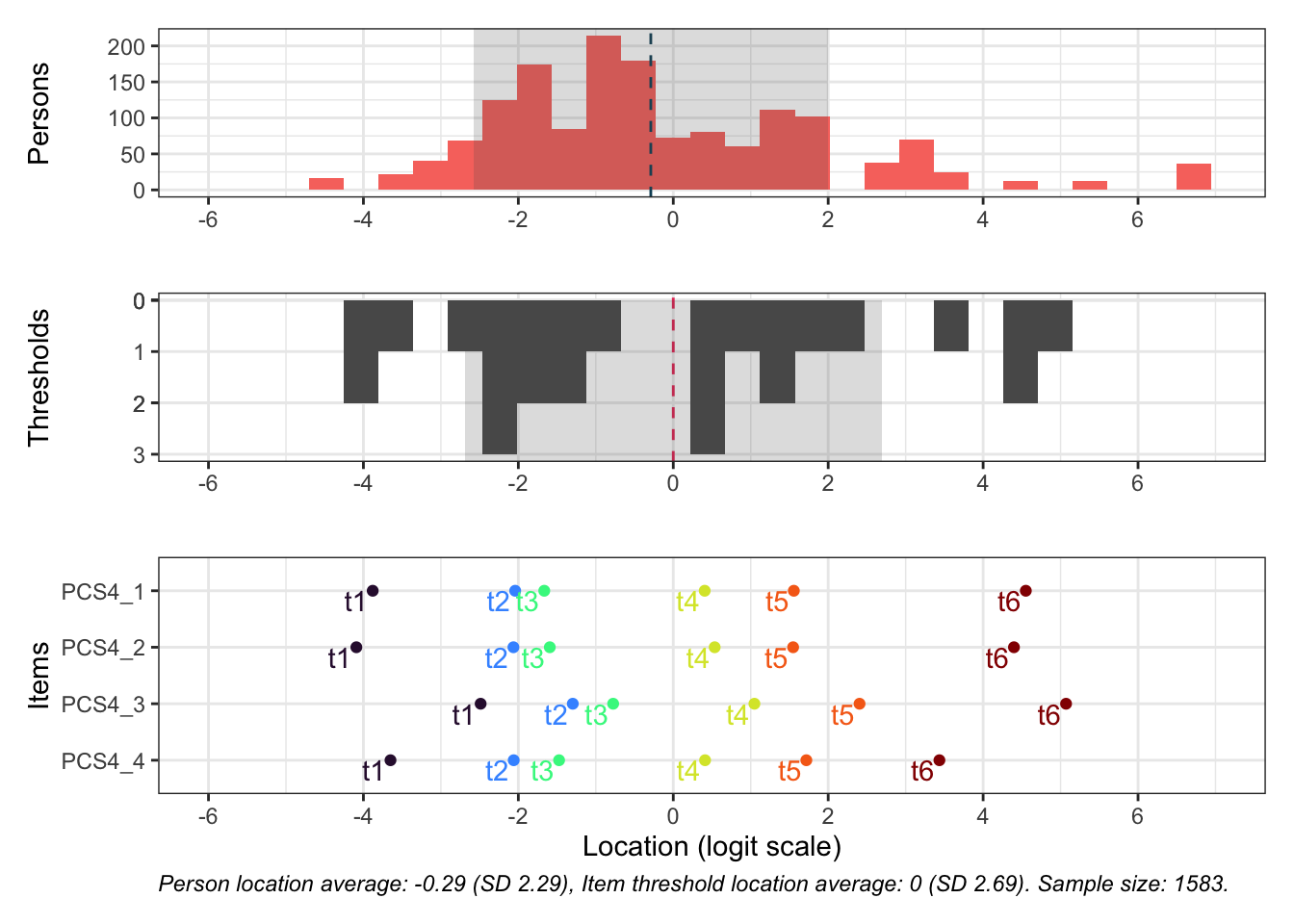
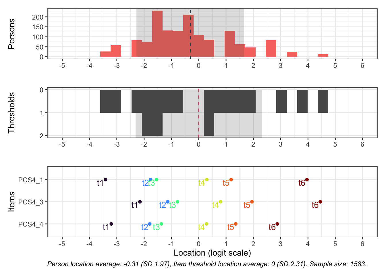
Code

# increase fig-height above as needed, if you have many items
RItargeting(d)

Code

RIitemHierarchy(d)

Code

RIdifTable(d, dif.time)

Item	2	4	5	Mean location	StDev	MaxDiff
PCS4_1	-0.222	-0.327	0.089	-0.153	0.216	0.416
PCS4_2	0.089	-0.152	-0.387	-0.150	0.238	0.476
PCS4_3	0.360	0.777	0.516	0.551	0.211	0.417
PCS4_4	-0.228	-0.298	-0.218	-0.248	0.044	0.080

Code

RIdifFigTime(d, dif.time) + coord_cartesian(ylim = c(-4,4))

Code

partgam_DIF(as.data.frame(d),dif.time)

    Item      Var   gamma     se pvalue padj.BH sig   lower   upper
1 PCS4_1 dif.time -0.1092 0.0368 0.0030  0.0120   * -0.1814 -0.0371
2 PCS4_2 dif.time  0.0495 0.0418 0.2365  0.9460     -0.0325  0.1315
3 PCS4_3 dif.time  0.1212 0.0352 0.0006  0.0023  **  0.0522  0.1901
4 PCS4_4 dif.time -0.0112 0.0375 0.7660  1.0000     -0.0847  0.0624

Response categories are surprisingly well-behaved, considering the lack of labels.

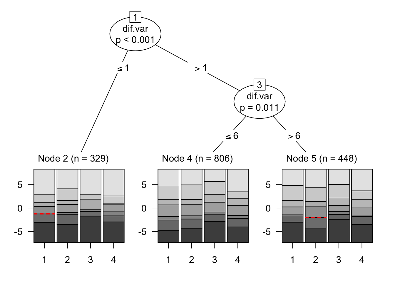
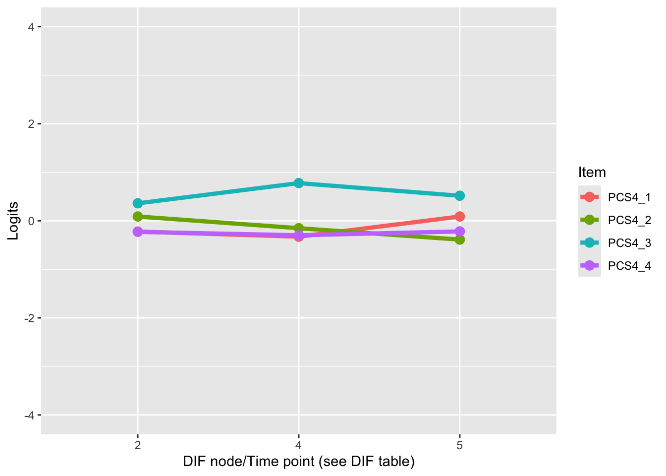
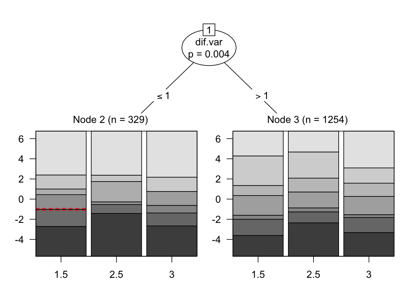
DIF over time is not problematic.

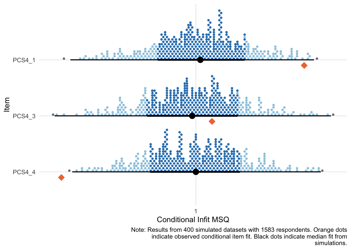
Item 2 has low fit and problematic residual correlations. This is not surprising considering its very general content regarding the latent construct.

PCS4_2 “Jag har förmågan att hantera min psykiska ohälsa nu”

We’ll remove item 2.

Code

d$PCS4_2 <- NULL

3.3 Rasch analysis 2

itemnr	item
PCS4_1	Jag känner mig säker på min förmåga att hantera min psykiska ohälsa
PCS4_3	Jag kan på egen hand hantera min psykiska ohälsa
PCS4_4	Jag känner att jag kan ta mig an de svårigheter det innebär att hantera min psykiska ohälsa

Code

simfit2 <- RIgetfit(d, iterations = 400, cpu = 8) 

RIitemfit(d, simfit2)

Item	InfitMSQ	Infit thresholds	OutfitMSQ	Outfit thresholds	Infit diff	Outfit diff	Relative location
PCS4_1	1.06	[0.931, 1.065]	1.043	[0.926, 1.067]	no misfit	no misfit	0.10
PCS4_3	1.009	[0.922, 1.075]	1.008	[0.919, 1.076]	no misfit	no misfit	0.83
PCS4_4	0.926	[0.932, 1.069]	0.909	[0.931, 1.078]	0.006	0.022	0.00
Note:
MSQ values based on conditional calculations (n = 1583 complete cases). Simulation based thresholds from 400 simulated datasets.

Code

RIgetfitPlot(simfit2, d)

Code

RIrestscore(d)

Item	Observed value	Model expected value	Absolute difference	Adjusted p-value (BH)	Statistical significance level	Location	Relative location
PCS4_1	0.71	0.69	0.02	0.316		-0.21	0.10
PCS4_3	0.71	0.69	0.02	0.316		0.52	0.83
PCS4_4	0.74	0.69	0.05	0.003	**	-0.31	0.00

Code

RIbootRestscore(d, samplesize = 600, cpu = 8, iterations = 250)

Item	Item-restscore result	% of iterations	Conditional MSQ infit	Relative average item location
PCS4_4	overfit	34	0.93	0
Note:
Results based on 250 bootstrap iterations with n = 600 and 3 items. Conditional mean-square infit based on complete responders only (n = 1583).

Code

RIpcmPCA(d)

PCA of Rasch model residuals
Eigenvalues	Proportion of variance
1.56	54.4%
1.44	45.4%
0.00	0.1%

Code

simcor <- RIgetResidCor(d,500,8)
RIresidcorr(d, simcor$p99)

	PCS4_1	PCS4_3
PCS4_1
PCS4_3	-0.49
PCS4_4	-0.41	-0.4
Note:
Relative cut-off value is -0.372, which is 0.061 above the average correlation (-0.433). Correlations above the cut-off are highlighted in red text.

Code

RIloadLoc(d)

Code

mirt(d, model=1, itemtype='Rasch', verbose = FALSE) %>% 
  plot(type="trace", as.table = TRUE, 
       theta_lim = c(-6,6))

Code

# increase fig-height above as needed, if you have many items
RItargeting(d)

Code

RIitemHierarchy(d)

Code

RIdifTable(d, dif.time)

Item	2	3	Mean location	StDev	MaxDiff
PCS4_1	-0.172	-0.203	-0.188	0.022	0.032
PCS4_3	0.356	0.495	0.425	0.099	0.139
PCS4_4	-0.184	-0.292	-0.238	0.076	0.108

Code

RIdifFigTime(d, dif.time) + coord_cartesian(ylim = c(-4,4))

Code

partgam_DIF(as.data.frame(d),dif.time)

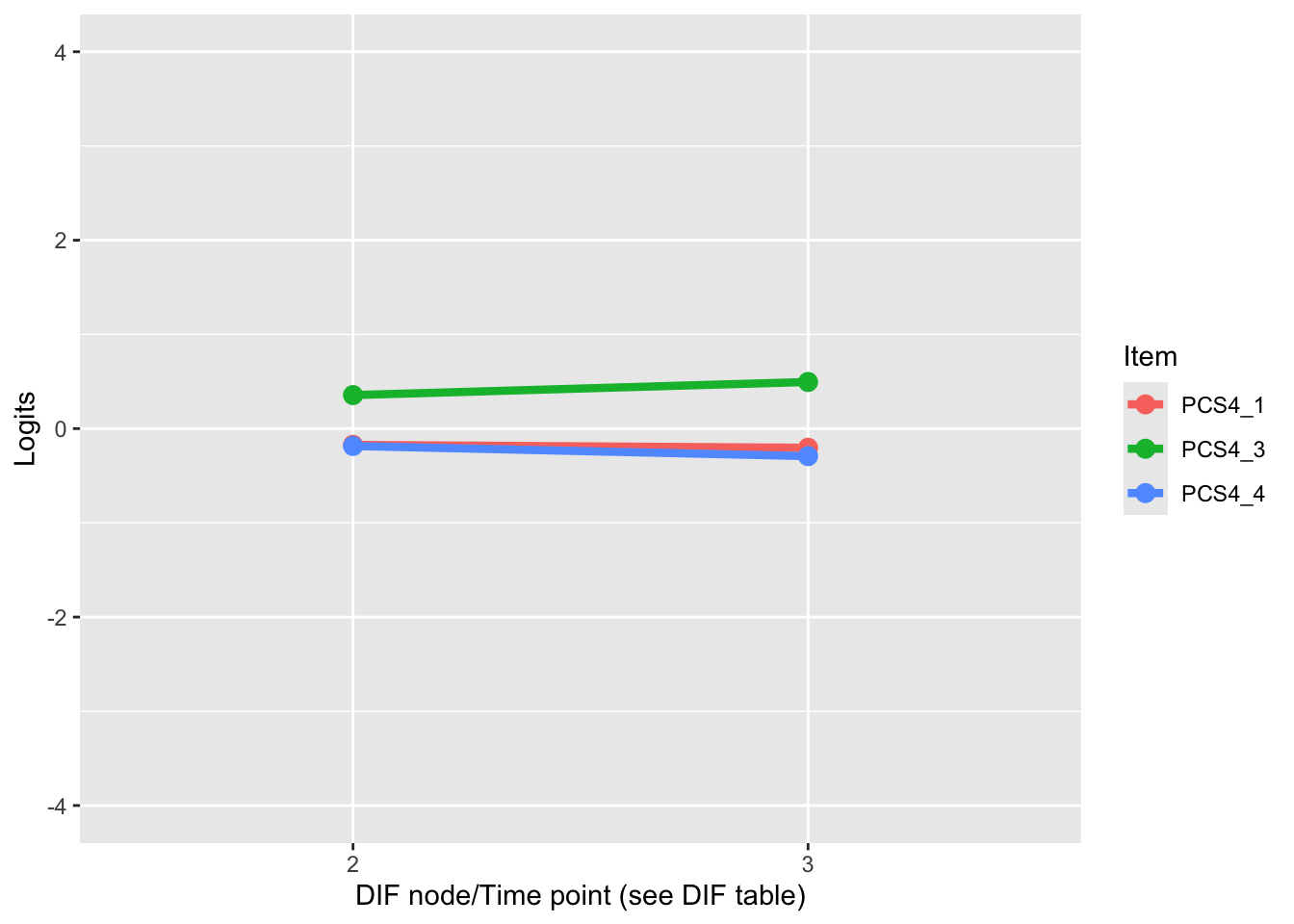
    Item      Var   gamma     se pvalue padj.BH  sig   lower   upper
1 PCS4_1 dif.time -0.1232 0.0357 0.0006  0.0017   ** -0.1932 -0.0531
2 PCS4_3 dif.time  0.1529 0.0347 0.0000  0.0000  ***  0.0850  0.2208
3 PCS4_4 dif.time  0.0037 0.0379 0.9230  1.0000      -0.0706  0.0780

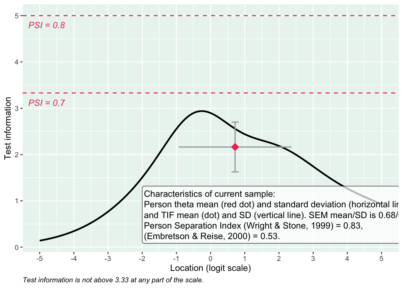
3.3.0.1 Reliability

Code

RItif(d, samplePSI = TRUE)

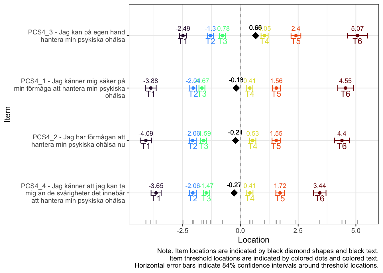
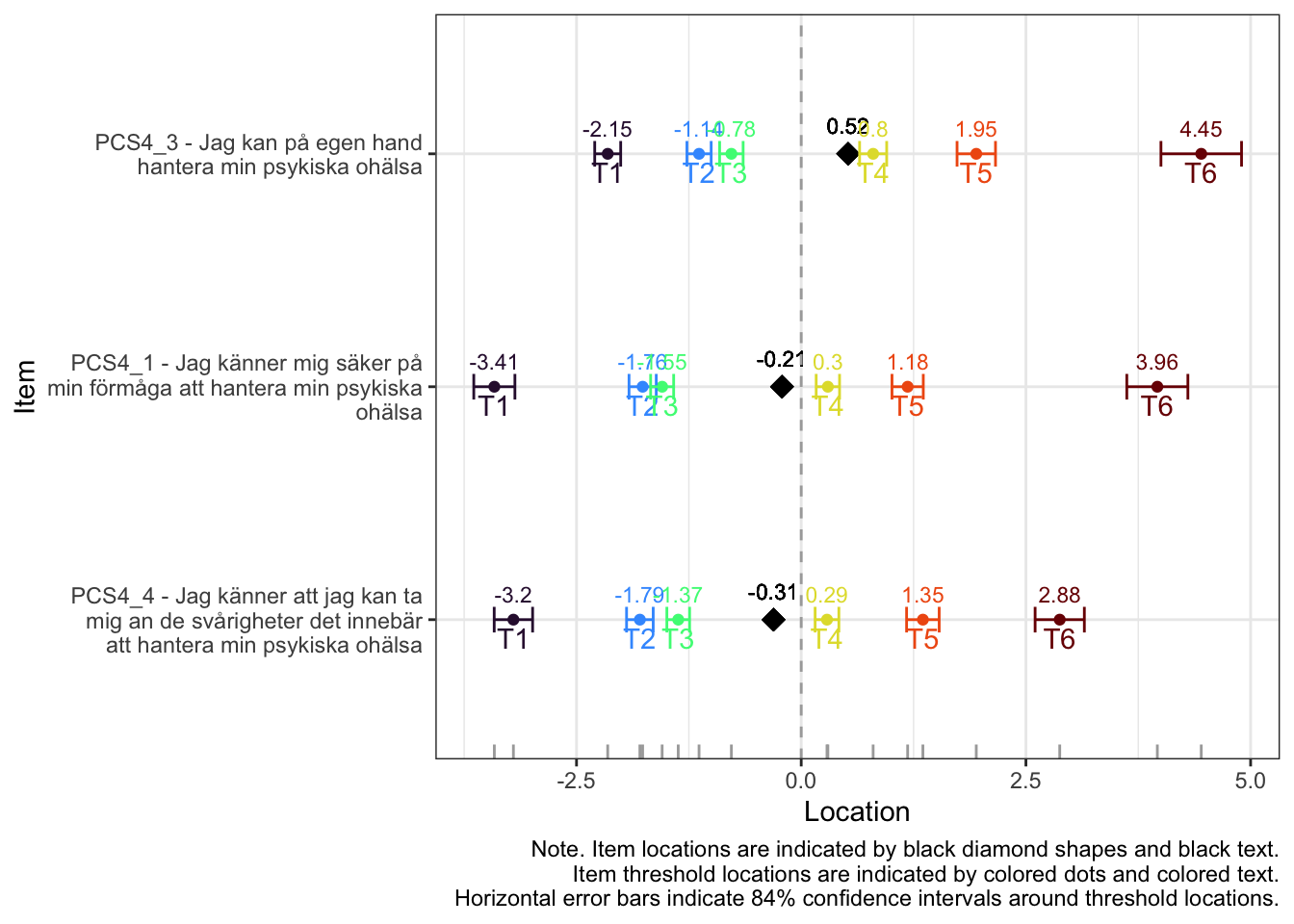
Relatively small distances between thresholds 2 and 3.

Item 4 is overdiscriminating slighly (low fit and high observed value in item-restscore). Bootstrapped item-restscore indicates low levels of issues as well. No problematic residual correlations. PSI is 0.83 with item 4 included.

PCS4_4 “Jag känner att jag kan ta mig an de svårigheter det innebär att hantera min psykiska ohälsa”

3.4 Item parameters

Code

RIitemparams(d, output = "file", filename = "PCS3_params.csv")
RIscoreSE(d)

Ordinal sum score	Logit score	Logit std.error
0	-4.924	0.723
1	-3.583	0.863
2	-2.873	0.780
3	-2.385	0.694
4	-2.001	0.637
5	-1.667	0.605
6	-1.351	0.592
7	-1.031	0.593
8	-0.690	0.604
9	-0.309	0.621
10	0.110	0.641
11	0.544	0.662
12	0.981	0.686
13	1.439	0.719
14	1.953	0.769
15	2.580	0.841
16	3.385	0.941
17	4.384	1.014
18	5.884	0.796

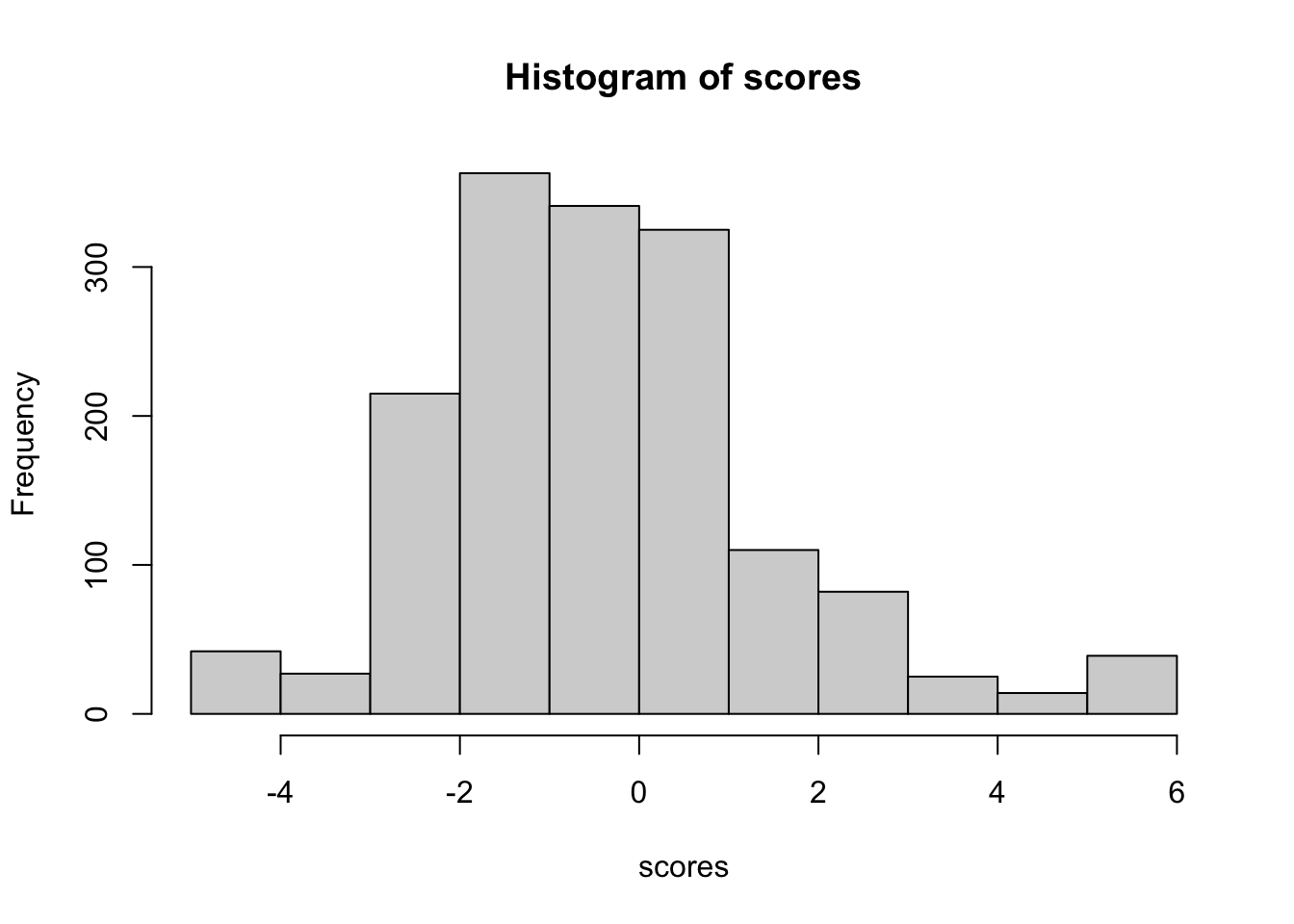
3.5 Latent score

Code

items <- RIitemparams(d,output = "dataframe") %>% 
  select(!Location) %>% 
  as.matrix()

scores <- RIestThetasCATr(d, items, theta_range = c(-8,8))
hist(scores)

Code

summary(scores)

   Min. 1st Qu.  Median    Mean 3rd Qu.    Max. 
-4.9233 -1.3505 -0.3089 -0.3125  0.9814  5.8843

Code

data.frame(PID = PID,
           time = dif.time,
           PCS_score = scores) %>% 
  write_csv("PCS3_score.csv")