Using Rasch and WLS to account for measurement uncertainties in regression models

Author

Affiliation

Magnus Johansson

Published

October 17, 2023

1 Introduction

There are several reasons for putting this blog post together. The larger issue is to investigate ways to analyze relationships between measures that have varying levels of measurement uncertainty across their respective range or continuum. This is relevant to any kind of latent variable measurement that uses multiple indicators/items/questions as a way to assess a latent variable.

In classical test theory (CTT; i.e. factor analysis) the assumption is generally that the measurement error is a single value, constant across the scale and across participants. Modern test theory (Rasch Measurement Theory (RMT) or Item Response Theory (IRT)) has tools to describe the varying uncertainties of the measure itself, and also allows for estimation of measurement uncertainty for each individual, based on the item properties.

In the “business-as-usual” approach, no matter which types of measurement uncertainty are ignored. The simple case of have two variables and an ordinary least squares (OLS) linear regression model will take the input from each variable as a perfect measurement. Bayesians may have another take on this, and I will look into that at a later point, so for now this is relevant for frequentist statistics.

“Business-as-usual” also makes use of ordinal sum scores disguised as interval scores. There is a seemingly wide-spread idea that estimated person interval scores is not significantly different from ordinal sum scores, and we’ll look further into that as well by including ordinal sum scores.

One way to take measurement uncertainty into account in a linear regression model is to use Weighted Least Squares (WLS) instead of OLS. However, this approach only allows weights for one variable. The weights will be based on the measurement uncertainty for the interval scores.

Additionally, we will use Quantile Regression, with and without weights.

2 Data

Data were collected for a project evaluating multiple work environment questionnaires. Two of the analyzed scales will be used in our example, as a foundation for simulated data. More information is available at the GitHub repository and website.

The two questionnaires cover the domains of “recovery” and “agency”, where the latter refers to workers’ perceived control over their work situation. Our analyses will look at how “agency” affects “recovery”. We will retain an interval scale score for the “recovery” scale throughout, while varying the “agency” between ordinal sum score, interval score, and interval score with weights, and check how these three reproduce the true simulated relationship between the two scales.

Variables will be named SEM for standard error of measurement, Theta for interval theta/scores/locations, and SumScore for ordinal sum scores.

We’ll also add analyses using structural equation modeling and weighted sum scores (based on confirmatory factor analysis factor loadings).

Code

library(RISEkbmRasch)
library(easystats)
library(quantreg)
library(faux)
library(broom.mixed)
library(lavaan)
library(DescTools)
library(lme4)

### some commands exist in multiple packages, here we define preferred ones that are frequently used
select <- dplyr::select
count <- dplyr::count
recode <- car::recode
rename <- dplyr::rename

3 Simulating data n = 800

We’ll pretend that we have n = 400 that are measured at two time points, with a specified correlation between measurements of 0.5. The difference in group means is set to 1 logit, and the standard deviation will be 1 logit for both points of measurement.

Code

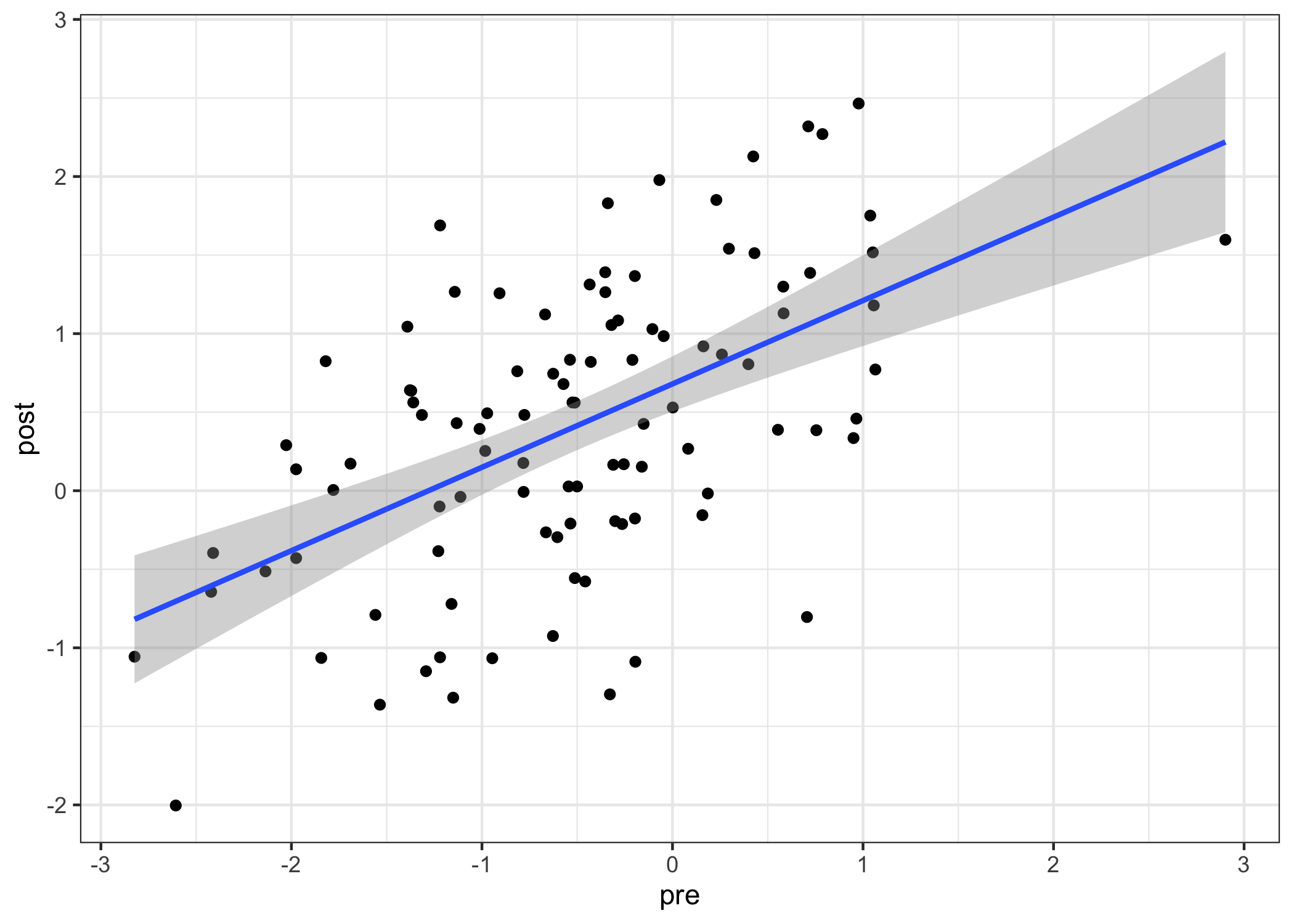
set.seed(1523)
n <- 100
data <- rnorm_multi(n = n, 
                  mu = c(-0.5, +0.5),
                  sd = c(1, 1),
                  r = c(0.5), 
                  varnames = c("pre", "post"),
                  empirical = FALSE)

cor_test("pre", "post", data = data)

Parameter1 | Parameter2 |    r |       95% CI | t(98) |         p
-----------------------------------------------------------------
pre        |       post | 0.55 | [0.39, 0.67] |  6.49 | < .001***

Observations: 100

Code

# light wrangling to get long format and an id variable
data_long <- data %>% 
  add_column(id = 1:(nrow(.))) %>% 
  pivot_longer(cols = c("pre", "post"), 
               names_to = "time", 
               values_to = "theta") %>% 
  mutate(theta = round(theta, 4),
         time = dplyr::recode(time, "pre" = 0, "post" = 1))
#write_csv(data, "data800simPrePost.csv")

3.1 Scatter plot

Code

data %>% 
  ggplot(aes(x = pre, y = post)) +
  geom_point() +
  geom_smooth(method = "lm", se = TRUE) +
  theme_bw()

3.2 Reference LMM results from the simulated theta values

Code

lmm0 <- lmer(scale(theta) ~ time + (1 | id), data = data_long) 

lmm0 %>%
  tidy(conf.int = TRUE) %>% 
  mutate(across(where(is.numeric), round, 4))

# A tibble: 4 × 8
  effect   group    term         estimate std.error statistic conf.low conf.high
  <chr>    <chr>    <chr>           <dbl>     <dbl>     <dbl>    <dbl>     <dbl>
1 fixed    <NA>     (Intercept)    -0.436    0.0902     -4.83   -0.613    -0.259
2 fixed    <NA>     time            0.872    0.0857     10.2     0.704     1.04 
3 ran_pars id       sd__(Interc…    0.668   NA          NA      NA        NA    
4 ran_pars Residual sd__Observa…    0.606   NA          NA      NA        NA

Code

icc(lmm0)

# Intraclass Correlation Coefficient

    Adjusted ICC: 0.548
  Unadjusted ICC: 0.444

Code

StdCoef(lmm0)

            Estimate* Std. Error*  df
(Intercept) 0.0000000  0.00000000 196
time        0.4370146  0.04297825 196
attr(,"class")
[1] "coefTable" "matrix"

The standardized coefficient of time is 0.424. This will be our reference value for comparison with the other analyses since ordinal sum scores and estimated theta scores will not be on the same scale.

3.3 Simulating polytomous data

Prepare the input item parameters.

Code

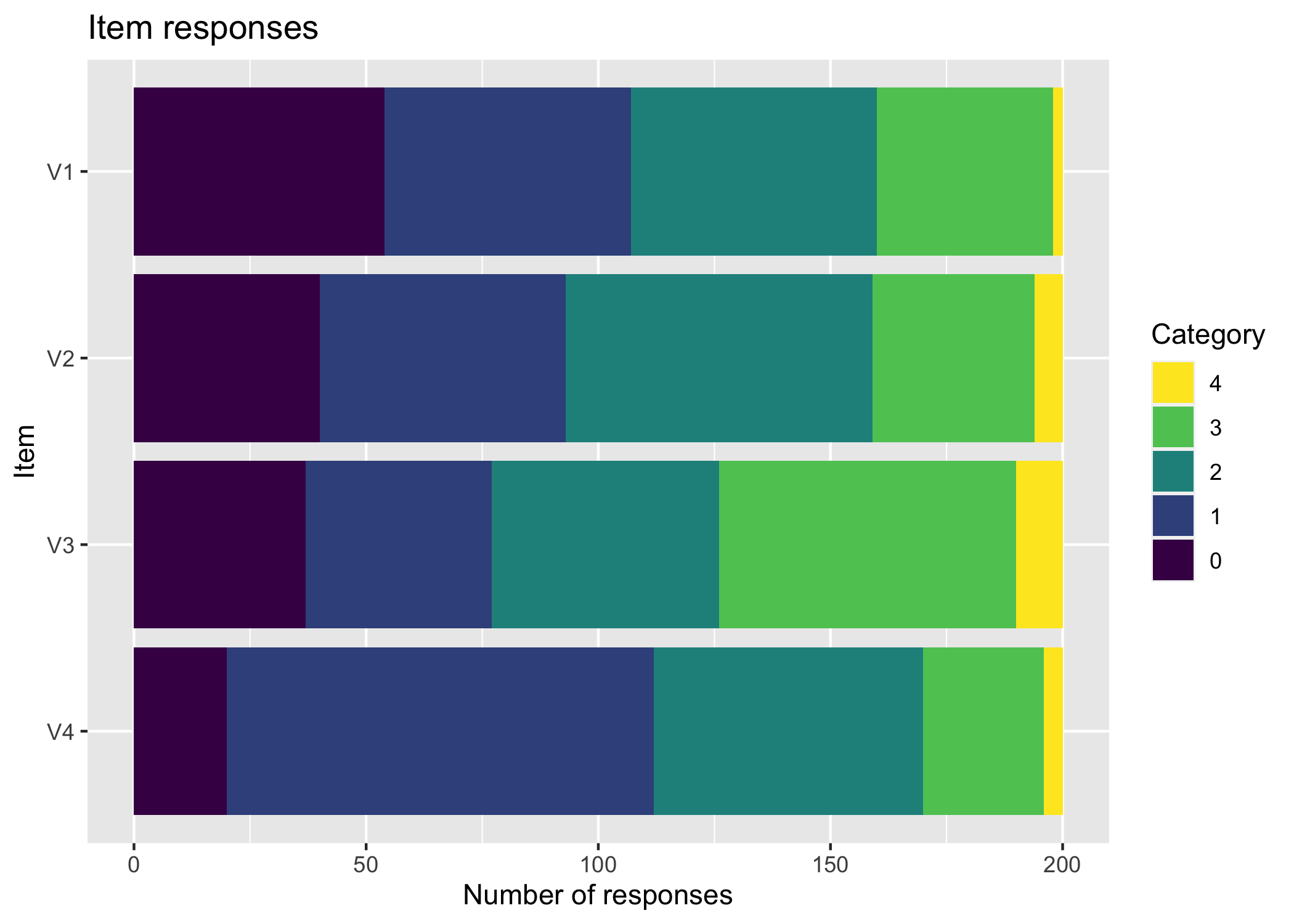
# item parameters
agencyParams <- read_csv("AgencyItemParameters.csv") %>% 
  as.matrix()

# put item parameters for agency into a list object
colnames(agencyParams) <- NULL

tlist <- lapply(1:nrow(agencyParams), function(i) {
  as.list(agencyParams[i, ])
})

# simulate polytomous data
simData <- SimPartialScore(
  deltaslist = tlist,
  thetavec = data_long$theta
) %>%
  as.data.frame()

A brief look at the simulated data.

Code

# distribution
RIbarstack(simData)

Code

# reliability/test information
RItif(simData, cutoff = 2.5, samplePSI = TRUE)

TIF 2.5 = PSI 0.6

3.4 Classical test theory

Confirmatory factor analysis (CFA) is used to estimate model fit.

Code

# specify model
cfa1 <- 'agencyCFA =~ V1 + V2 + V3 + V4'
# estimate model
cfa1.fit <- cfa(cfa1, 
                ordered = TRUE, 
                estimator = "DWLS",
                data = simData)
# get fit indices etc
summary(cfa1.fit, fit.measures = TRUE)

lavaan 0.6.15 ended normally after 13 iterations

  Estimator                                       DWLS
  Optimization method                           NLMINB
  Number of model parameters                        20

  Number of observations                           200

Model Test User Model:
                                                      
  Test statistic                                 1.426
  Degrees of freedom                                 2
  P-value (Chi-square)                           0.490

Model Test Baseline Model:

  Test statistic                               441.330
  Degrees of freedom                                 6
  P-value                                        0.000

User Model versus Baseline Model:

  Comparative Fit Index (CFI)                    1.000
  Tucker-Lewis Index (TLI)                       1.004

Root Mean Square Error of Approximation:

  RMSEA                                          0.000
  90 Percent confidence interval - lower         0.000
  90 Percent confidence interval - upper         0.127
  P-value H_0: RMSEA <= 0.050                    0.639
  P-value H_0: RMSEA >= 0.080                    0.209

Standardized Root Mean Square Residual:

  SRMR                                           0.023

Parameter Estimates:

  Standard errors                             Standard
  Information                                 Expected
  Information saturated (h1) model        Unstructured

Latent Variables:
                   Estimate  Std.Err  z-value  P(>|z|)
  agencyCFA =~                                        
    V1                1.000                           
    V2                0.918    0.109    8.403    0.000
    V3                1.179    0.138    8.542    0.000
    V4                0.942    0.110    8.576    0.000

Intercepts:
                   Estimate  Std.Err  z-value  P(>|z|)
   .V1                0.000                           
   .V2                0.000                           
   .V3                0.000                           
   .V4                0.000                           
    agencyCFA         0.000                           

Thresholds:
                   Estimate  Std.Err  z-value  P(>|z|)
    V1|t1            -0.613    0.095   -6.438    0.000
    V1|t2             0.088    0.089    0.987    0.323
    V1|t3             0.842    0.101    8.310    0.000
    V1|t4             2.326    0.265    8.791    0.000
    V2|t1            -0.842    0.101   -8.310    0.000
    V2|t2            -0.088    0.089   -0.987    0.323
    V2|t3             0.824    0.101    8.180    0.000
    V2|t4             1.881    0.178   10.583    0.000
    V3|t1            -0.896    0.103   -8.694    0.000
    V3|t2            -0.292    0.090   -3.240    0.001
    V3|t3             0.332    0.091    3.661    0.000
    V3|t4             1.645    0.150   10.980    0.000
    V4|t1            -1.282    0.121  -10.576    0.000
    V4|t2             0.151    0.089    1.692    0.091
    V4|t3             1.036    0.109    9.547    0.000
    V4|t4             2.054    0.205   10.020    0.000

Variances:
                   Estimate  Std.Err  z-value  P(>|z|)
   .V1                0.507                           
   .V2                0.585                           
   .V3                0.315                           
   .V4                0.563                           
    agencyCFA         0.493    0.074    6.682    0.000

Scales y*:
                   Estimate  Std.Err  z-value  P(>|z|)
    V1                1.000                           
    V2                1.000                           
    V3                1.000                           
    V4                1.000

Code

# get standardized factor loadings
inspect(cfa1.fit,what="std")$lambda

   agnCFA
V1  0.702
V2  0.644
V3  0.828
V4  0.661

Code

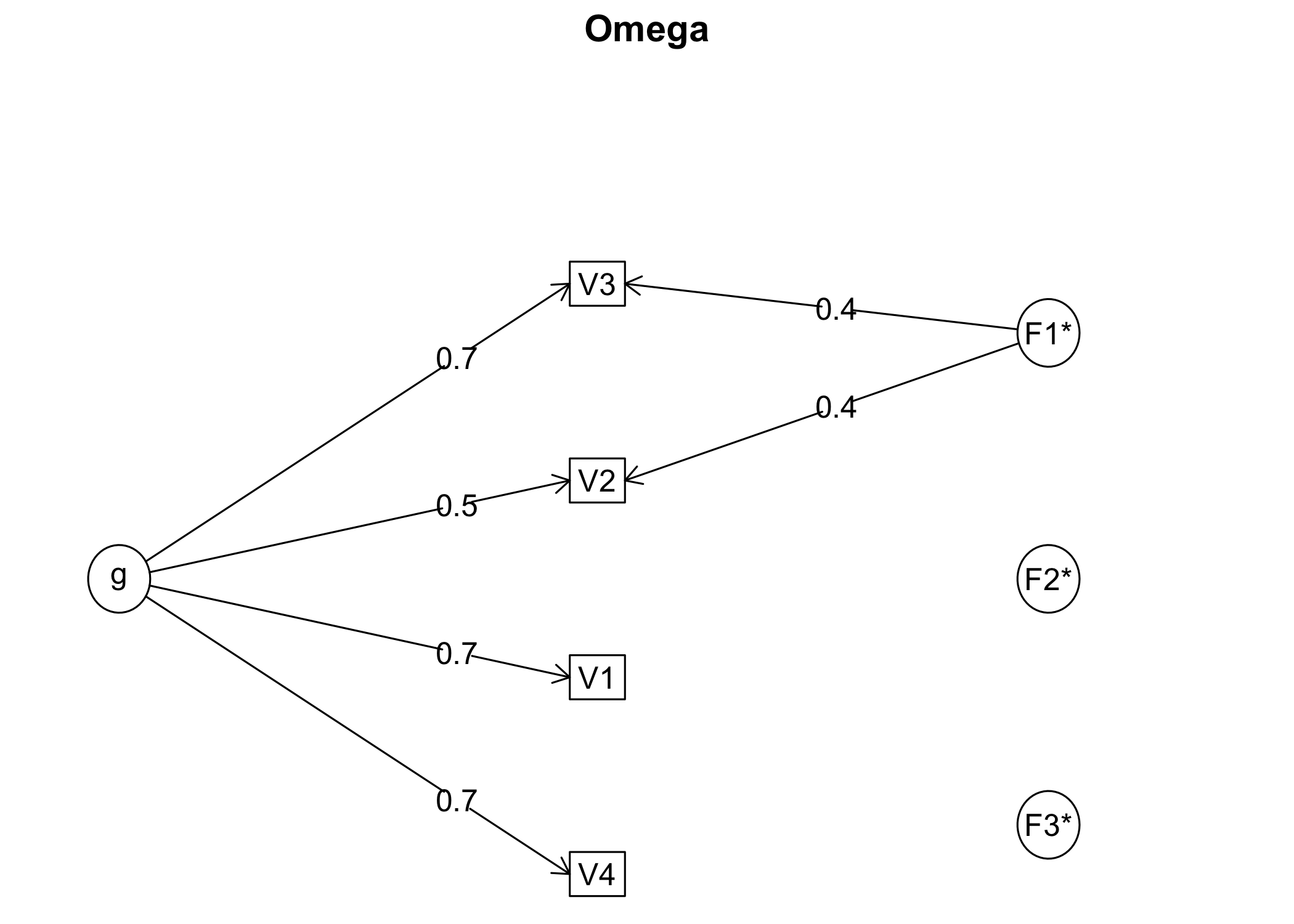
# save factor loadings to a vector
cfa1_loadings <- inspect(cfa1.fit,what="std")$lambda %>% 
  as.data.frame() %>% 
  pull(agencyCFA)

# CTT reliability
psych::alpha(simData)


Reliability analysis   
Call: psych::alpha(x = simData)

  raw_alpha std.alpha G6(smc) average_r S/N   ase mean   sd median_r
      0.76      0.76    0.72      0.45 3.2 0.027  1.6 0.83     0.45

    95% confidence boundaries 
         lower alpha upper
Feldt     0.71  0.76  0.81
Duhachek  0.71  0.76  0.82

 Reliability if an item is dropped:
   raw_alpha std.alpha G6(smc) average_r S/N alpha se  var.r med.r
V1      0.70      0.71    0.62      0.44 2.4    0.035 0.0071  0.46
V2      0.72      0.73    0.64      0.47 2.7    0.033 0.0010  0.46
V3      0.66      0.67    0.57      0.40 2.0    0.041 0.0024  0.40
V4      0.73      0.73    0.65      0.48 2.7    0.033 0.0047  0.51

 Item statistics 
     n raw.r std.r r.cor r.drop mean   sd
V1 200  0.77  0.77  0.65   0.57  1.4 1.11
V2 200  0.75  0.74  0.61   0.53  1.6 1.09
V3 200  0.83  0.81  0.74   0.64  1.9 1.20
V4 200  0.71  0.74  0.60   0.52  1.5 0.91

Non missing response frequency for each item
      0    1    2    3    4 miss
V1 0.27 0.26 0.26 0.19 0.01    0
V2 0.20 0.26 0.33 0.17 0.03    0
V3 0.18 0.20 0.24 0.32 0.05    0
V4 0.10 0.46 0.29 0.13 0.02    0

Code

psych::omega(simData)

Omega 
Call: omegah(m = m, nfactors = nfactors, fm = fm, key = key, flip = flip, 
    digits = digits, title = title, sl = sl, labels = labels, 
    plot = plot, n.obs = n.obs, rotate = rotate, Phi = Phi, option = option, 
    covar = covar)
Alpha:                 0.76 
G.6:                   0.72 
Omega Hierarchical:    0.7 
Omega H asymptotic:    0.89 
Omega Total            0.78 

Schmid Leiman Factor loadings greater than  0.2 
      g   F1* F2* F3*   h2   u2   p2
V1 0.73               0.49 0.51 1.08
V2 0.52  0.39         0.43 0.57 0.62
V3 0.66  0.45         0.64 0.36 0.69
V4 0.66               0.41 0.59 1.04

With Sums of squares  of:
   g  F1*  F2*  F3* 
1.67 0.36 0.00 0.00 

general/max  4.69   max/min =   Inf
mean percent general =  0.86    with sd =  0.24 and cv of  0.28 
Explained Common Variance of the general factor =  0.82 

The degrees of freedom are -3  and the fit is  0 
The number of observations was  200  with Chi Square =  0  with prob <  NA
The root mean square of the residuals is  0 
The df corrected root mean square of the residuals is  NA

Compare this with the adequacy of just a general factor and no group factors
The degrees of freedom for just the general factor are 2  and the fit is  0.06 
The number of observations was  200  with Chi Square =  11.68  with prob <  0.0029
The root mean square of the residuals is  0.08 
The df corrected root mean square of the residuals is  0.13 

RMSEA index =  0.155  and the 10 % confidence intervals are  0.078 0.248
BIC =  1.08 

Measures of factor score adequacy             
                                                 g   F1* F2*   F3*
Correlation of scores with factors            0.86  0.60   0  0.08
Multiple R square of scores with factors      0.73  0.36   0  0.01
Minimum correlation of factor score estimates 0.46 -0.28  -1 -0.99

 Total, General and Subset omega for each subset
                                                 g  F1* F2*  F3*
Omega total for total scores and subscales    0.78 0.69  NA 0.66
Omega general for total scores and subscales  0.70 0.46  NA 0.66
Omega group for total scores and subscales    0.08 0.23  NA 0.00

3.5 Estimate person thetas/latent scores

Next step is to estimate person thetas/scores/locations based on the pre-specified item parameters.

Code

# estimate person thetas
personThetas <- RIestThetas(simData,itemParams = agencyParams)
# estimate person theta SEM
personSEM <- map_vec(personThetas, ~ catR::semTheta(.x, it = agencyParams, method = "WL", model = "PCM"))
# add person thetas to the simulated data
simData$estTheta <- personThetas
simData$estSEM <- personSEM
# add ordinal sum scores to the simulated data
simData <- simData %>% 
  mutate(SumScore = V1+V2+V3+V4)
# add weighted ordinal sum scores to the simulated data
simData$weightedSumScore <- simData$V1*cfa1_loadings[1] + 
  simData$V2*cfa1_loadings[2] + 
  simData$V3*cfa1_loadings[3] + 
  simData$V4*cfa1_loadings[4]

# add simulated theta values to the simData
simData$simTheta <- data_long$theta
# add id variable
simData$id <- data_long$id
# create grouping variable for quintiles
simData$quintile <- as.factor(ntile(simData$simTheta, 5))

# add time variable to data
simData$time <- data_long$time

write_csv(simData, "simData.csv")

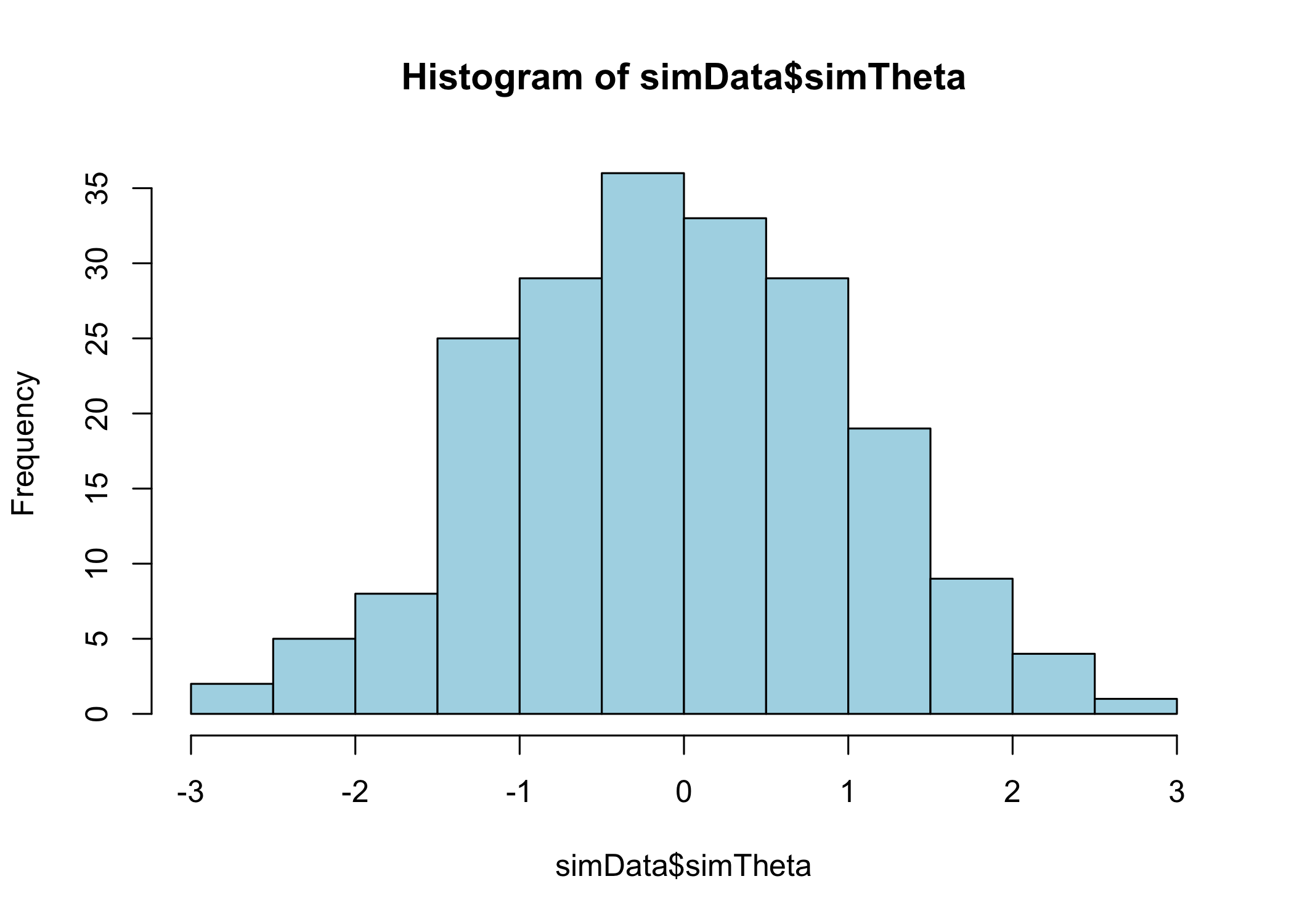
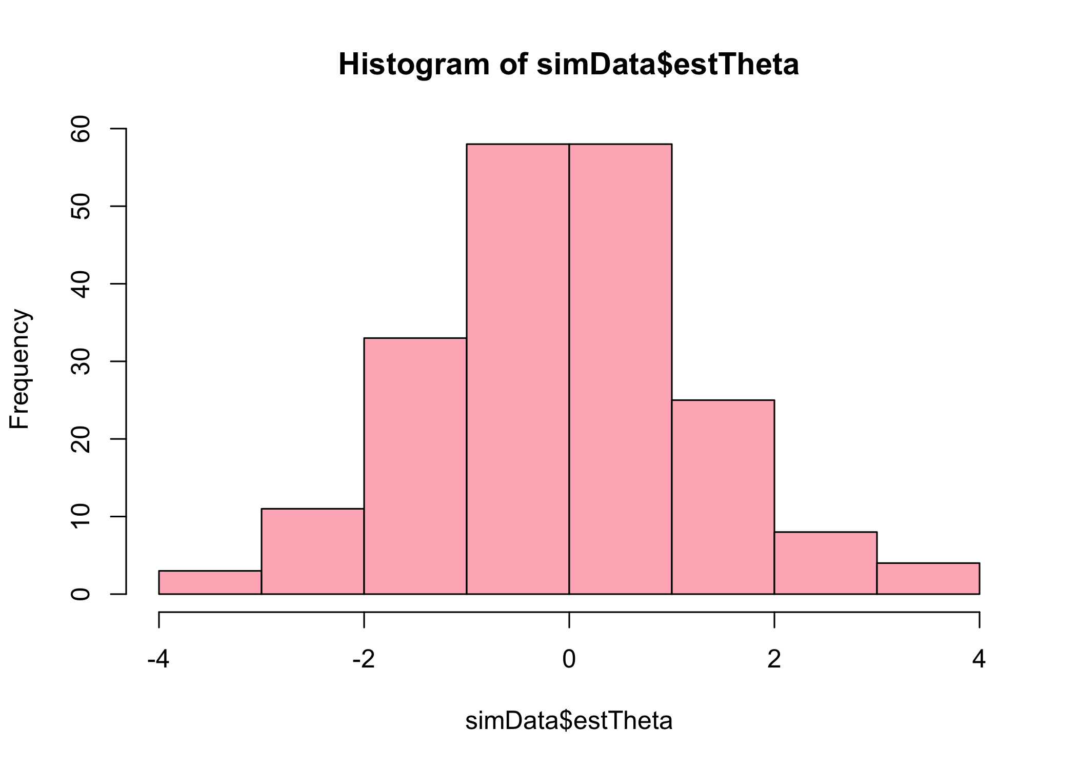
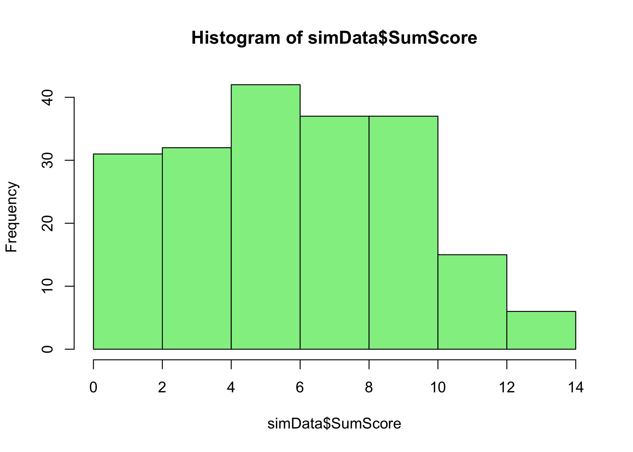
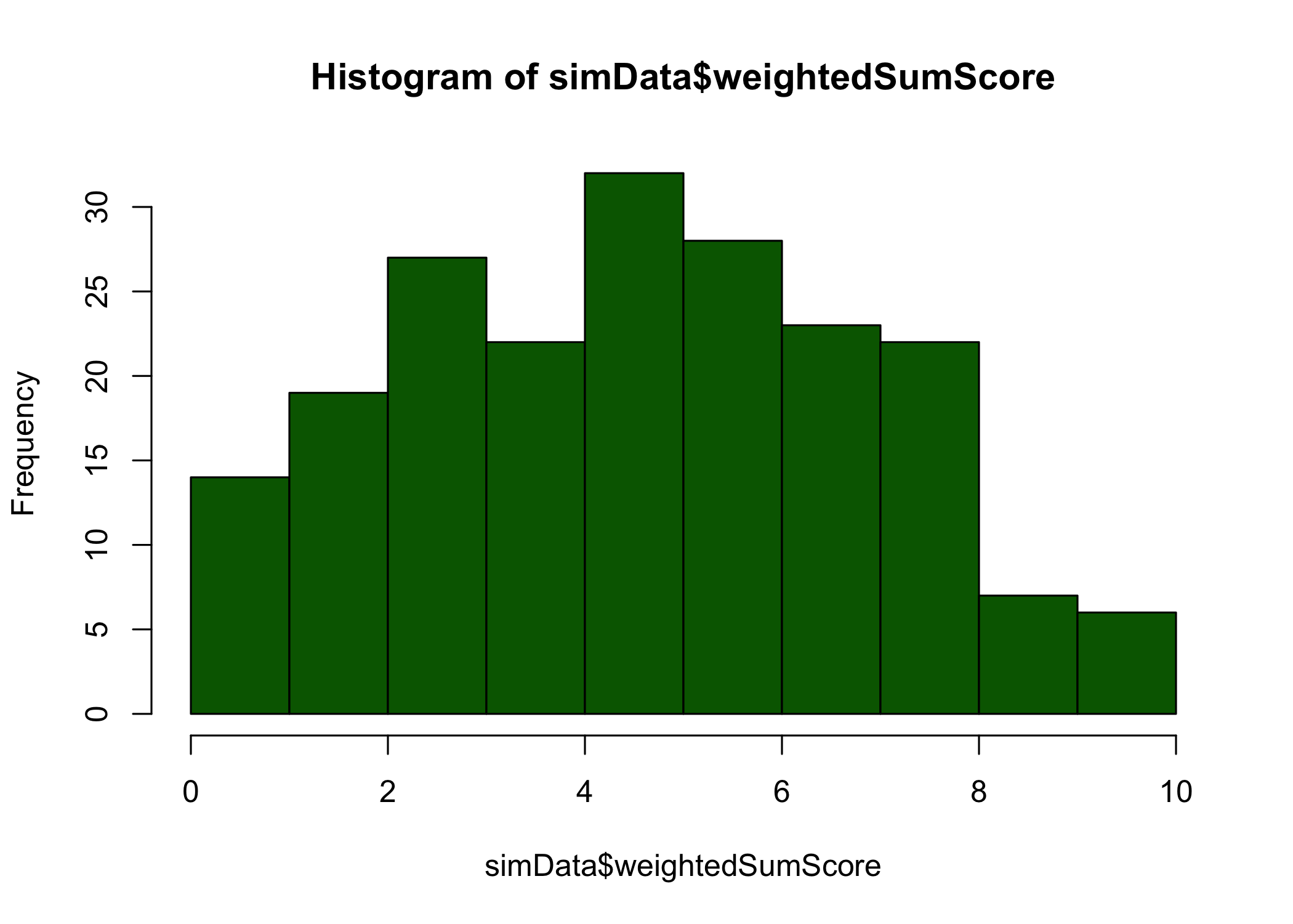
Code

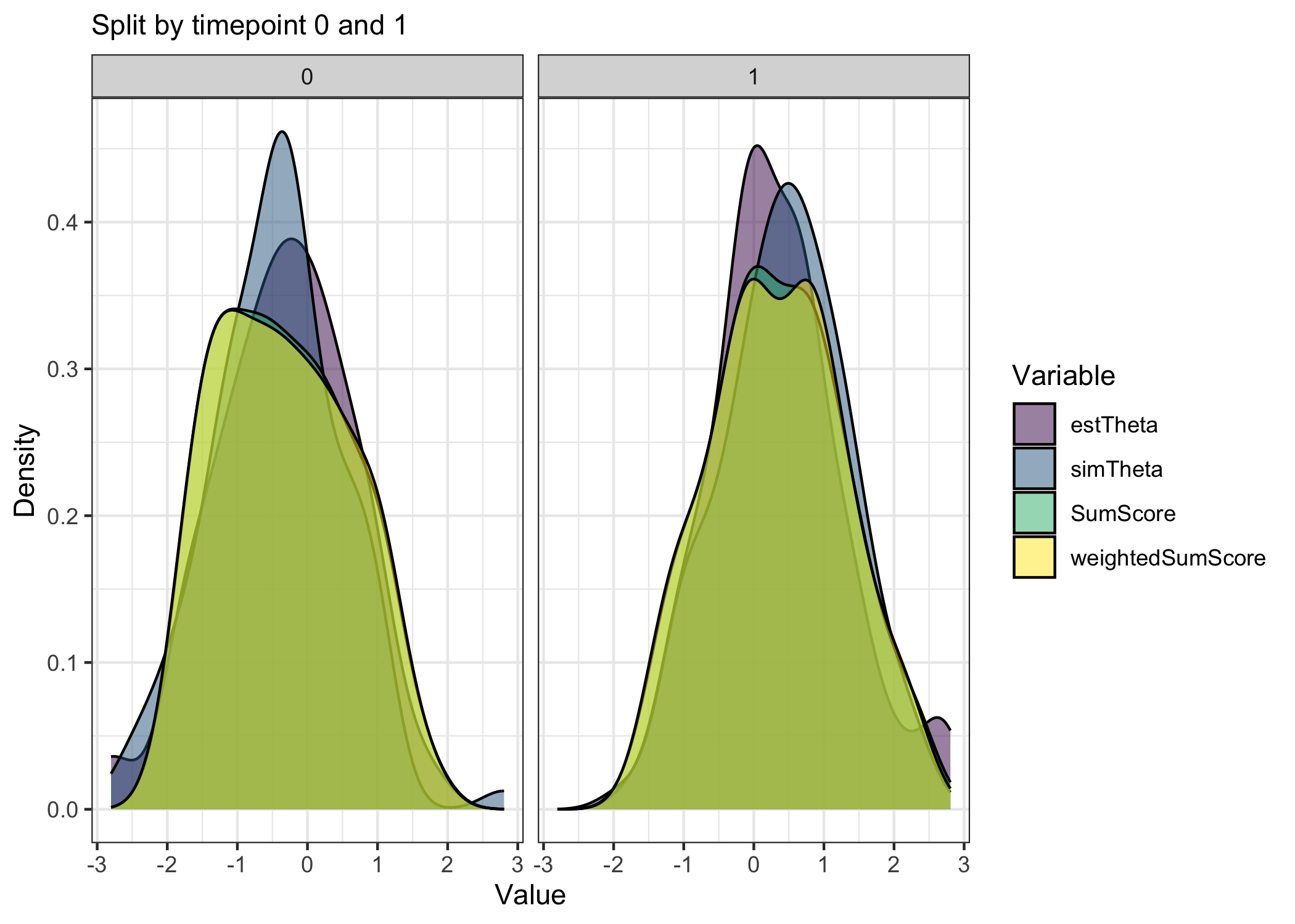
hist(simData$simTheta, col = "lightblue")
hist(simData$estTheta, col = "lightpink")
hist(simData$SumScore, col = "lightgreen")
hist(simData$weightedSumScore, col = "darkgreen")

Histograms of generated and estimated theta values, ordinal sum scores, and weighted ordinal sum scores

Code

# density plot for all four of the above histograms, facet_wrapped by time
simData %>% 
  mutate(across(c("simTheta", "estTheta", "SumScore", "weightedSumScore"), ~ scale(.x))) %>%
  pivot_longer(cols = c("simTheta", "estTheta", "SumScore", "weightedSumScore"), 
               names_to = "variable", 
               values_to = "value") %>% 
  ggplot(aes(x = value, fill = variable)) +
  geom_density(alpha = 0.5) +
  facet_wrap(~time) +
  theme_bw() +
  scale_fill_viridis_d() +
  labs(x = "Value", y = "Density", fill = "Variable",
       subtitle = "Split by timepoint 0 and 1")

Density plot of scaled values for all four variables

4 Statistical analyses

4.1 LMM with estimated theta

Code

lmm1 <- lmer(scale(estTheta) ~ time + (1 | id), data = simData) 

lmm1 %>%
  tidy(conf.int = TRUE) %>% 
  mutate(across(where(is.numeric), round, 4))

# A tibble: 4 × 8
  effect   group    term         estimate std.error statistic conf.low conf.high
  <chr>    <chr>    <chr>           <dbl>     <dbl>     <dbl>    <dbl>     <dbl>
1 fixed    <NA>     (Intercept)    -0.347    0.094      -3.70   -0.532    -0.163
2 fixed    <NA>     time            0.695    0.0998      6.96    0.499     0.890
3 ran_pars id       sd__(Interc…    0.620   NA          NA      NA        NA    
4 ran_pars Residual sd__Observa…    0.706   NA          NA      NA        NA

Code

icc(lmm1)

# Intraclass Correlation Coefficient

    Adjusted ICC: 0.436
  Unadjusted ICC: 0.383

Code

StdCoef(lmm1)

            Estimate* Std. Error*  df
(Intercept) 0.0000000   0.0000000 196
time        0.3481564   0.0500326 196
attr(,"class")
[1] "coefTable" "matrix"

0.37 (SE = 0.026) compared with 0.42.

4.2 Weighted LMM with estimated theta

We’ll use the estimated theta SEM as weights.

Code

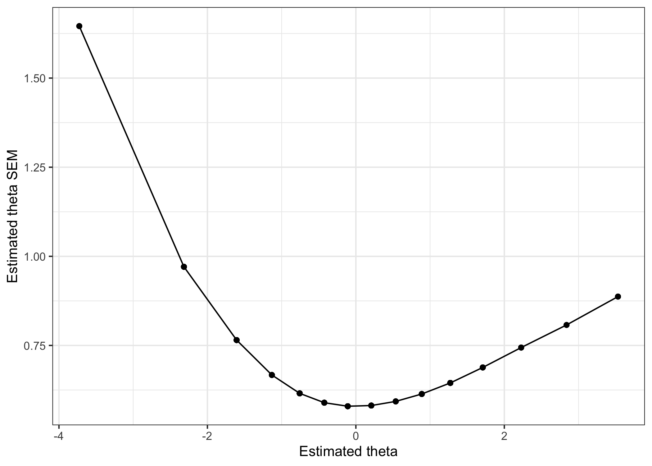
# plot range of estSEM across estTheta
simData %>% 
  ggplot(aes(x = estTheta, y = estSEM)) +
  geom_point() +
  geom_line(group = 1) +
  theme_bw() +
  labs(x = "Estimated theta", y = "Estimated theta SEM")

Plot of estimated theta SEM against estimated theta

Code

lmm2 <- lmer(scale(estTheta) ~ time + (1 | id), data = simData,
             weights = estSEM) 

lmm2 %>%
  tidy(conf.int = TRUE) %>% 
  mutate(across(where(is.numeric), round, 4))

# A tibble: 4 × 8
  effect   group    term         estimate std.error statistic conf.low conf.high
  <chr>    <chr>    <chr>           <dbl>     <dbl>     <dbl>    <dbl>     <dbl>
1 fixed    <NA>     (Intercept)    -0.429    0.101      -4.27   -0.626    -0.232
2 fixed    <NA>     time            0.798    0.0992      8.04    0.603     0.992
3 ran_pars id       sd__(Interc…    0.731   NA          NA      NA        NA    
4 ran_pars Residual sd__Observa…    0.571   NA          NA      NA        NA

Code

icc(lmm2)

# Intraclass Correlation Coefficient

    Adjusted ICC: 0.622
  Unadjusted ICC: 0.524

Code

StdCoef(lmm2)

            Estimate* Std. Error*  df
(Intercept)  0.000000  0.00000000 196
time         0.399825  0.04970946 196
attr(,"class")
[1] "coefTable" "matrix"

0.414 (SE = 0.026) compared with 0.42.

4.3 LMM with ordinal sum score

Code

lmm3 <- lmer(scale(SumScore) ~ time + (1 | id), data = simData)

lmm3 %>%
  tidy(conf.int = TRUE) %>% 
  mutate(across(where(is.numeric), round, 4))

# A tibble: 4 × 8
  effect   group    term         estimate std.error statistic conf.low conf.high
  <chr>    <chr>    <chr>           <dbl>     <dbl>     <dbl>    <dbl>     <dbl>
1 fixed    <NA>     (Intercept)    -0.336    0.0944     -3.57   -0.522    -0.152
2 fixed    <NA>     time            0.673    0.101       6.64    0.474     0.872
3 ran_pars id       sd__(Interc…    0.614   NA          NA      NA        NA    
4 ran_pars Residual sd__Observa…    0.717   NA          NA      NA        NA

Code

icc(lmm3)

# Intraclass Correlation Coefficient

    Adjusted ICC: 0.423
  Unadjusted ICC: 0.375

Code

StdCoef(lmm3)

            Estimate* Std. Error*  df
(Intercept) 0.0000000  0.00000000 196
time        0.3373715  0.05083355 196
attr(,"class")
[1] "coefTable" "matrix"

0.373 (SE = 0.026) compared with 0.42.

4.4 LMM with weighted ordinal sum score

Code

lmm4 <- lmer(scale(weightedSumScore) ~ time + (1 | id), data = simData)

lmm4 %>%
  tidy(conf.int = TRUE) %>% 
  mutate(across(where(is.numeric), round, 4))

# A tibble: 4 × 8
  effect   group    term         estimate std.error statistic conf.low conf.high
  <chr>    <chr>    <chr>           <dbl>     <dbl>     <dbl>    <dbl>     <dbl>
1 fixed    <NA>     (Intercept)    -0.333    0.0945     -3.53   -0.518    -0.148
2 fixed    <NA>     time            0.666    0.102       6.54    0.467     0.866
3 ran_pars id       sd__(Interc…    0.611   NA          NA      NA        NA    
4 ran_pars Residual sd__Observa…    0.720   NA          NA      NA        NA

Code

icc(lmm4)

# Intraclass Correlation Coefficient

    Adjusted ICC: 0.419
  Unadjusted ICC: 0.372

Code

StdCoef(lmm4)

            Estimate* Std. Error*  df
(Intercept) 0.0000000  0.00000000 196
time        0.3339848  0.05107553 196
attr(,"class")
[1] "coefTable" "matrix"

0.373 (SE = 0.026) compared with 0.424.

5 Summary

Code

# rbind together lmm0 to lmm4 in one dataframe
lmm_summary <- rbind(tidy(lmm0), tidy(lmm1), tidy(lmm2), tidy(lmm3), tidy(lmm4)) %>% 
  add_column(model = rep(c("lmm0", "lmm1estTheta", "lmm2weightedTheta", "lmm3sumscore", "lmm4weighted Sumscore"),each = 4))
lmm_summary %>% 
  filter(term == "time") %>% 
  write_csv(paste0(n,"_lmm_summary.csv"))

Code

# check ICC vs correlation pre/post for estTheta
simData %>% 
  mutate(time = factor(time, labels = c("pre","post"))) %>% 
  pivot_wider(names_from = time, values_from = estTheta, id_cols = "id") %>% 
  cor_test("pre","post")

Parameter1 | Parameter2 |    r |       95% CI | t(98) |         p
-----------------------------------------------------------------
pre        |       post | 0.44 | [0.26, 0.58] |  4.80 | < .001***

Observations: 100

Reuse

https://creativecommons.org/licenses/by/4.0/

Citation

BibTeX citation:

@online{johansson2023,
  author = {Magnus Johansson},
  title = {Using {Rasch} and {WLS} to Account for Measurement
    Uncertainties in Regression Models},
  date = {2023-10-17},
  url = {https://pgmj.github.io/compLatent.html},
  langid = {en}
}

For attribution, please cite this work as:

Magnus Johansson. (2023, October 17). Using Rasch and WLS to account for measurement uncertainties in regression models. https://pgmj.github.io/compLatent.html