When one uses Rasch or Item Response Theory to estimate measurement values on the latent scale it is also easy to estimate an “individualized” measurement error for each value estimated. It has been suggested that a useful way to use this output when analyzing data with two repeated measurement points is to conduct one paired t-test for each individual, comparing the pre/post measurements and using their respective measurement error as the “population standard error” (Hobart et al., 2010).
This strategy results in measurably detectable change for individuals across two time points. Whether this change is meaningful requires external validation to determine. Since measurement error is not equal across the continuum, how large the measurably detactable change is will also vary depending on the pre-measurement value.
All the usual limitations and caveats with t-tests apply. This post is not an endorsement of using multiple t-tests as a primary strategy of analysis, but it may be an interesting perspective that takes measurement error into account and focuses on individual outcomes.
Note
This is work in progress and will be updated and expanded on. The first aim is to share code to do individual t-tests of theta+SEM and summarise the results. Later on, we’ll look at other methods to analyze longitudinal data, both looking at group level and individual level change.
The reliability of the scale/test will of course heavily influence the possibility of detecting change over time. In the Rasch Measurement Theory and Item Response Theory paradigm, reliability is not a single point value that is constant across the latent continuum (REF to separate post on reliability). Depending on the item threshold locations, the test has varying reliability.
Later in this post, I will present a figure describing the Test Information Function, and then a figure with the SEM values across the latent continuum.
As shown in the separate post on reliability (LINK), SEM * 1.96 will contain the true value in 95% of cases.
We could use the parameters from the input, but to add some real world usage to the setup, we’ll stack the response data and estimate the item threshold locations using the eRm package with the Partial Credig Model and Conditional Maximum Likelihood.
Code
erm_item_parameters<-RIitemparams(td, output ="dataframe")%>%select(!Location)%>%rename(T1 =`Threshold 1`, T2 =`Threshold 2`, T3 =`Threshold 3`)%>%as.matrix()# center item parameters to sum = 0erm_item_parameters<-erm_item_parameters-mean(erm_item_parameters)
2.3 Estimating person locations and SEM
Using Weighted Likelihood (Warm, 1989) to minimize bias.
Code
# estimate thetas/person locations, based on eRm estimated item thresholdserm_thetas<-RIestThetas(td, itemParams =erm_item_parameters)# estimate measurement error (SEM)erm_sem<-map_vec(erm_thetas, ~catR::semTheta(.x, it =erm_item_parameters, method ="WL", model ="PCM"))d_long$erm_thetas<-erm_thetasd_long$erm_sem<-erm_sem
3 Change
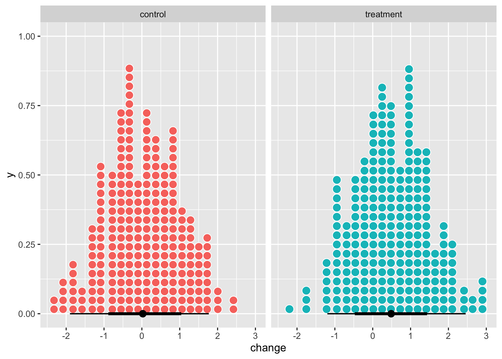
How many have changed 0.5+ logits (the mean change simulated, also corresponding to 0.5 SD) in the generated data? This could serve as a reference.
Only using t1 and t3 estimated person locations/thetas and SEM values.
Code
d_wide_tt<-d_long%>%pivot_wider(values_from =c(erm_thetas,erm_sem), id_cols =c(id,group), names_from =time)%>%mutate(id =as.numeric(id))# basic formula for t-test# (d_wide_tt$erm_thetas_1[1] - d_wide_tt$erm_thetas_3[1]) / sqrt(d_wide_tt$erm_sem_1[1] + d_wide_tt$erm_sem_3[1])# t-tests for all rows in dataframet_values<-c()for(iin1:nrow(d_wide_tt)){t_values[i]<-(d_wide_tt$erm_thetas_3[i]-d_wide_tt$erm_thetas_1[i])/sqrt(d_wide_tt$erm_sem_3[i]+d_wide_tt$erm_sem_1[i])}data.frame(t_values =t_values, group =rep(c("Intervention","Control"), each =250))%>%mutate(result =case_when(t_values>1.96~"Improved",t_values<-1.96~"Worsened",TRUE~"No detectable change"))%>%group_by(group)%>%count(result)%>%kbl_rise(tbl_width =40)%>%row_spec(c(1,4),bold=TRUE)
group
result
n
Control
Improved
12
Control
No detectable change
229
Control
Worsened
9
Intervention
Improved
27
Intervention
No detectable change
219
Intervention
Worsened
4
4.1 “Recovery” of n changed
Again, strongly affected by precision/reliability
References
Hobart, J. C., Cano, S. J., & Thompson, a. J. (2010). Effect sizes can be misleading: Is it time to change the way we measure change? Journal of Neurology, Neurosurgery and Psychiatry, 81(9), 1044. https://doi.org/10.1136/jnnp.2009.201392
---title: "Analyzing individual change with t-tests"author: name: Magnus Johansson affiliation: RISE Research Institutes of Sweden affiliation-url: https://www.ri.se/sv/vad-vi-gor/expertiser/kategoriskt-baserade-matningar orcid: 0000-0003-1669-592Xdate: last-modifiedcitation: type: 'webpage'csl: apa.cslexecute: cache: true warning: false message: falseeditor: markdown: wrap: 72editor_options: chunk_output_type: consolebibliography: ttest.bib---## IntroductionWhen one uses Rasch or Item Response Theory to estimate measurement values on the latent scale it is also easy to estimate an "individualized" measurement error for each value estimated. It has been suggested that a useful way to use this output when analyzing data with two repeated measurement points is to conduct one paired t-test for each individual, comparing the pre/post measurements and using their respective measurement error as the "population standard error" [@hobart_effect_2010].This strategy results in measurably detectable change for individuals across two time points. Whether this change is meaningful requires external validation to determine. Since measurement error is not equal across the continuum, how large the measurably detactable change is will also vary depending on the pre-measurement value.All the usual limitations and caveats with t-tests apply. This post is not an endorsement of using multiple t-tests as a primary strategy of analysis, but it may be an interesting perspective that takes measurement error into account and focuses on individual outcomes.::: {.callout-note}This is work in progress and will be updated and expanded on. The first aim is to share code to do individual t-tests of theta+SEM and summarise the results. Later on, we'll look at other methods to analyze longitudinal data, both looking at group level and individual level change.:::The reliability of the scale/test will of course heavily influence the possibility of detecting change over time. In the Rasch Measurement Theory and Item Response Theory paradigm, reliability is not a single point value that is constant across the latent continuum (REF to separate post on reliability). Depending on the item threshold locations, the test has varying reliability. Later in this post, I will present a figure describing the Test Information Function, and then a figure with the SEM values across the latent continuum.As shown in the separate post on reliability (LINK), SEM * 1.96 will contain the true value in 95% of cases.```{r}library(tidyverse)library(eRm)library(janitor)library(RISEkbmRasch)library(lme4)library(modelsummary)library(broom.mixed)library(marginaleffects)library(faux)library(ggdist)### some commands exist in multiple packages, here we define preferred ones that are frequently usedselect <- dplyr::selectcount <- dplyr::countrecode <- car::recoderename <- dplyr::renametheme_rise <-function(fontfamily ="Lato", axissize =13, titlesize =15,margins =12, axisface ="plain", panelDist =0.6, ...) {theme_minimal() +theme(text =element_text(family = fontfamily),axis.title.x =element_text(margin =margin(t = margins),size = axissize ),axis.title.y =element_text(margin =margin(r = margins),size = axissize ),plot.title =element_text(face ="bold",size = titlesize ),axis.title =element_text(face = axisface ),plot.caption =element_text(face ="italic" ),legend.text =element_text(family = fontfamily),legend.background =element_rect(color ="lightgrey"),strip.background =element_rect(color ="lightgrey"),panel.spacing =unit(panelDist, "cm", data =NULL),panel.border =element_rect(color ="grey", fill =NA), ... )}theme_set(theme_rise())```## Simulating longitudinal data3 time points for later use. First, we'll focus on t1 and t3 and run the t-tests focusing on individual change.```{r}set.seed(1523)data_g1 <-rnorm_multi(n =250, mu =c(-0.25, 0, 0.25),sd =c(1, 1, 1),r =c(0.5), varnames =c("t_1", "t_2", "t_3"),empirical =FALSE) %>%add_column(group ="treatment") %>%rownames_to_column("id")data_g2 <-rnorm_multi(n =250, mu =c(-0.25, -0.15, -0.05),sd =c(1, 1, 1),r =c(0.5), varnames =c("t_1", "t_2", "t_3"),empirical =FALSE) %>%add_column(group ="control") %>%mutate(id =c(251:500))d <-rbind(data_g1,data_g2)d_long <- d %>%pivot_longer(starts_with("t")) %>%mutate(time =as.numeric(gsub("t_","",name))) %>%select(!name)```### Simulate response data```{r}# item list for simulationtlist <-list(t1 =list(1.2, 1.8, 2.4),t2 =list(-1.3, -0.5, 0.5),t3 =list(-0.3, 0.3, 1.2),t4 =list(0.1, 0.6, 1.6),t5 =list(-0.3, 0.7, 1.5),t6 =list(-1.6, -1, -0.3),t7 =list(1, 1.8, 2.5),t8 =list(-1.3, -0.7, 0.4),t9 =list(-0.8, 1.4, 1.9),t10 =list(0.25, 1.25, 2.15))inputDeltas <-tibble(q1 =c(1.2, 1.8, 2.4),q2 =c(-1.3, -0.5, 0.5),q3 =c(-0.3, 0.3, 1.2),q4 =c(0.1, 0.6, 1.6),q5 =c(-0.3, 0.7, 1.5),q6 =c(-1.6, -1, -0.3),q7 =c(1, 1.8, 2.5),q8 =c(-1.3, -0.7, 0.4),q9 =c(-0.8, 1.4, 1.9),q10 =c(0.25, 1.25, 2.15)) %>%t() %>%as.data.frame() %>%mutate(Average =rowMeans(., na.rm = T)) %>%mutate_if(is.double, round, digits =2) %>%rownames_to_column(var ="Item") %>% dplyr::rename(T1 = V1,T2 = V2,T3 = V3)# simulate response data based on the above defined item thresholdstd <-SimPartialScore(deltaslist = tlist,thetavec = d_long$value) %>%as.data.frame()```### Estimating item threshold locationsWe could use the parameters from the input, but to add some real world usage to the setup, we'll stack the response data and estimate the item threshold locations using the `eRm` package with the Partial Credig Model and Conditional Maximum Likelihood.```{r}erm_item_parameters <-RIitemparams(td, output ="dataframe") %>%select(!Location) %>%rename(T1 =`Threshold 1`,T2 =`Threshold 2`,T3 =`Threshold 3`) %>%as.matrix()# center item parameters to sum = 0erm_item_parameters <- erm_item_parameters -mean(erm_item_parameters)```### Estimating person locations and SEMUsing Weighted Likelihood (Warm, 1989) to minimize bias.```{r}# estimate thetas/person locations, based on eRm estimated item thresholdserm_thetas <-RIestThetas(td, itemParams = erm_item_parameters)# estimate measurement error (SEM)erm_sem <-map_vec(erm_thetas, ~ catR::semTheta(.x, it = erm_item_parameters, method ="WL", model ="PCM"))d_long$erm_thetas <- erm_thetasd_long$erm_sem <- erm_sem```## ChangeHow many have changed 0.5+ logits (the mean change simulated, also corresponding to 0.5 SD) in the generated data? This could serve as a reference.```{r}d <- d %>%mutate(change = t_3 - t_1)summary(d$change)sd(d$change)sd(d$t_3)ggplot(d, aes(x = change, fill = group, color = group)) +#geom_histogram() +stat_dotsinterval(color ="black", slab_color ="white", slab_linewidth =0.5) +facet_wrap(~ group) +guides(fill ="none", color ="none")d %>%mutate(change_grp =case_when(change >0.5~"Improved > 0.5", change <-0.5~"Worsened > 0.5",TRUE~"In between")) %>%group_by(group) %>%count(change_grp) %>%kbl_rise(tbl_width =40) %>%row_spec(c(1,4),bold=TRUE)```### Test information function```{r}RItif(td, samplePSI =TRUE)```## t-tests of individual changeOnly using t1 and t3 estimated person locations/thetas and SEM values.```{r}d_wide_tt <- d_long %>%pivot_wider(values_from =c(erm_thetas,erm_sem),id_cols =c(id,group),names_from = time ) %>%mutate(id =as.numeric(id))# basic formula for t-test# (d_wide_tt$erm_thetas_1[1] - d_wide_tt$erm_thetas_3[1]) / sqrt(d_wide_tt$erm_sem_1[1] + d_wide_tt$erm_sem_3[1])# t-tests for all rows in dataframet_values <-c()for (i in1:nrow(d_wide_tt)) { t_values[i] <- (d_wide_tt$erm_thetas_3[i] - d_wide_tt$erm_thetas_1[i]) /sqrt(d_wide_tt$erm_sem_3[i] + d_wide_tt$erm_sem_1[i])}data.frame(t_values = t_values,group =rep(c("Intervention","Control"), each =250)) %>%mutate(result =case_when(t_values >1.96~"Improved", t_values <-1.96~"Worsened",TRUE~"No detectable change")) %>%group_by(group) %>%count(result) %>%kbl_rise(tbl_width =40) %>%row_spec(c(1,4),bold=TRUE)```### "Recovery" of n changedAgain, strongly affected by precision/reliability